From simulations to real data, on the relevance
of deep learning models and domain adaptation:
Application to astrophysics with CTAO and LST-1
PhD Thesis Defense, Michaël Dell'aiera
| Jury composed of | |
|
Giovanni Lamanna Marie Chabert Karl Kosack Alice Caplier |
David Rousseau Alexandre Benoit Thomas Vuillaume |



dellaiera.michael@gmail.com
Introduction
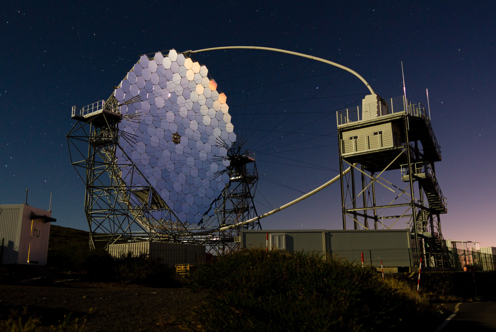
Cherenkov Telescope Array Observatory (CTAO)
**Exploring the Universe at Very High Energies (VHE)**
* Gamma-ray astronomy * Recent science * Success of H.E.S.S., MAGIC, VERITAS, Fermi-LAT, ... * CTAO * Next-generation ground-based observatory for gamma-ray astronomy * Increased sensitivity * First Large-Sized Telescope (LST) operational * GammaLearn project * Collaboration between LAPP (CNRS) and LISTIC * Fosters innovative methods in AI for CTAO * Evaluate the added value of deep learning * Open Science
[Science with the Cherenkov Telescope Array.](https://www.worldscientific.com/doi/abs/10.1142/10986) WORLD SCIENTIFIC, 2019 https://gammalearn.pages.in2p3.fr/gammalearn/
Gamma-ray astronomy
**Observation of the universe in the gamma-ray segment of the electromagnetic spectrum (> 0.1 MeV)**
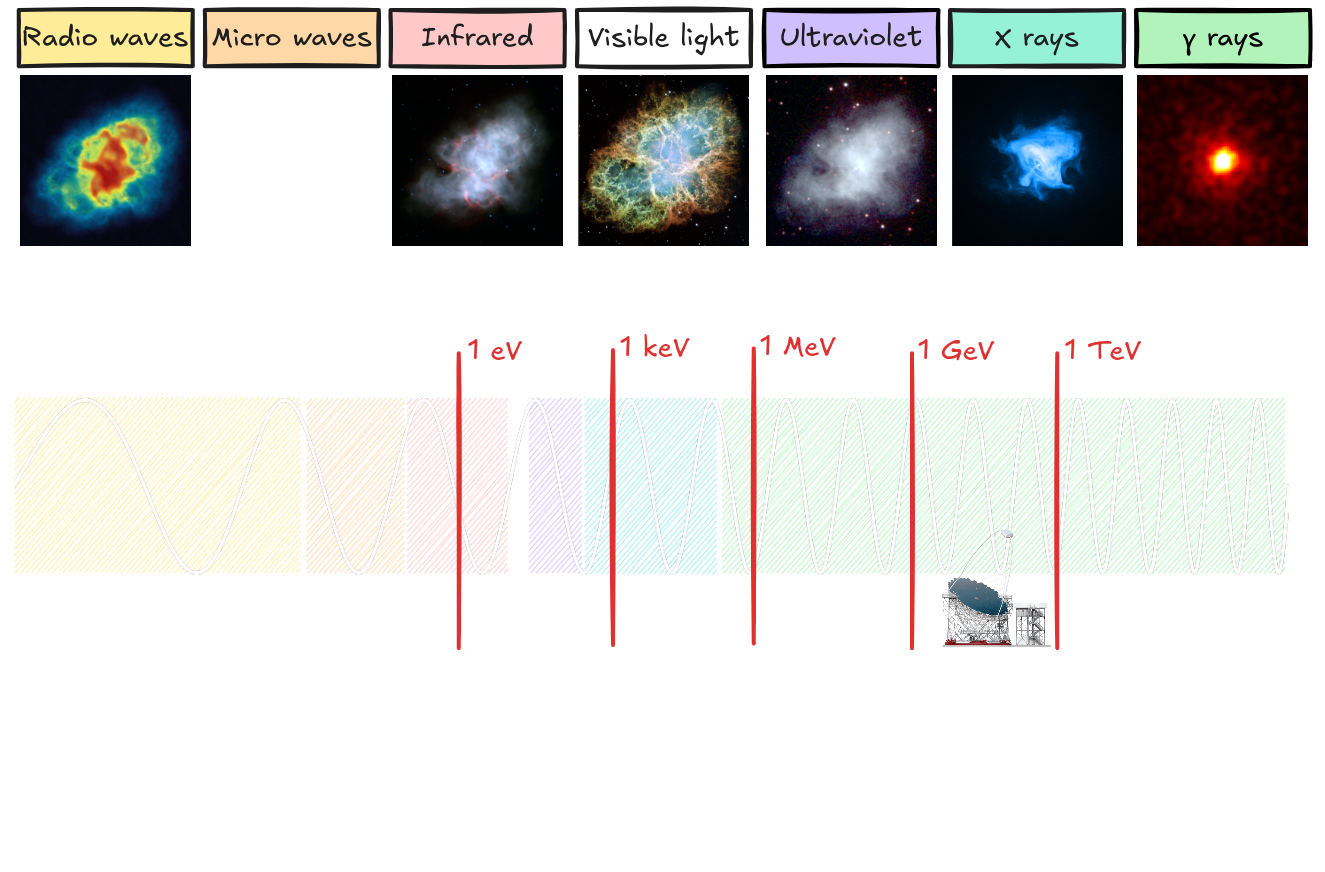
Energy ranges * CTAO: 20 GeV to 300 TeV * LST prevailing in the lowest energies Scientific objectives * Understanding the origin and role of relativistic cosmic particles * Probing extreme environments (e.g. black holes, neutron stars) * Multi-messenger analysis (neutrinos, gravitational waves and cosmic rays) * Exploring frontiers in physics (e.g. dark matter)
Werner Hofmann. “Perspectives from CTA in relativistic astrophysics”. In: Fourteenth Marcel Grossmann Meeting - MG14. Ed. by Massimo Bianchi, Robert T. Jansen, and Remo Ruffini. Jan. 2018, pp. 223–242
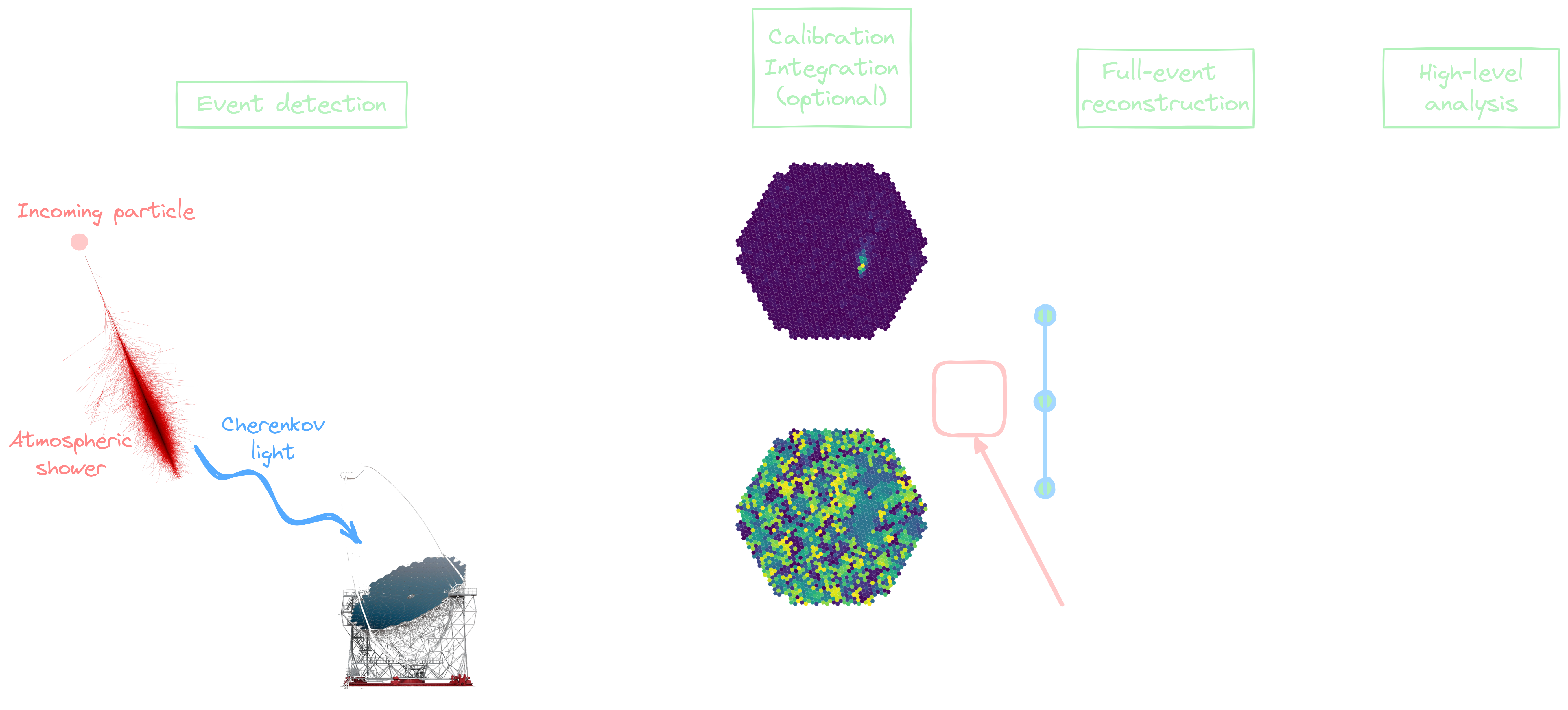
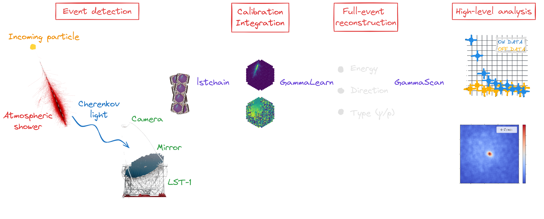
Reconstruction workflow
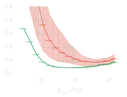
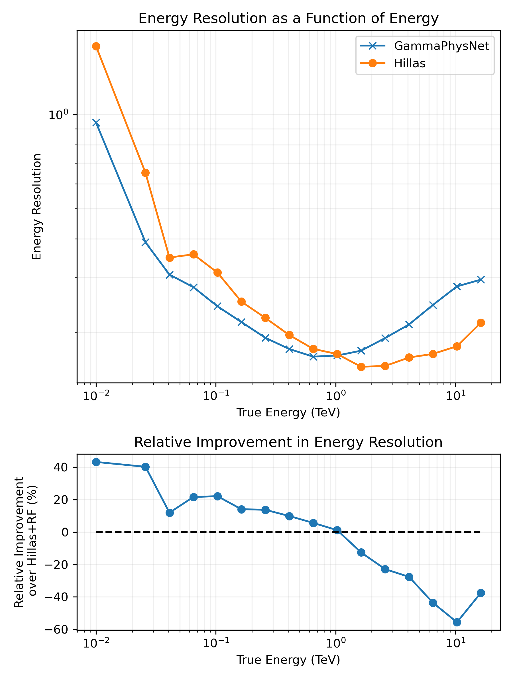
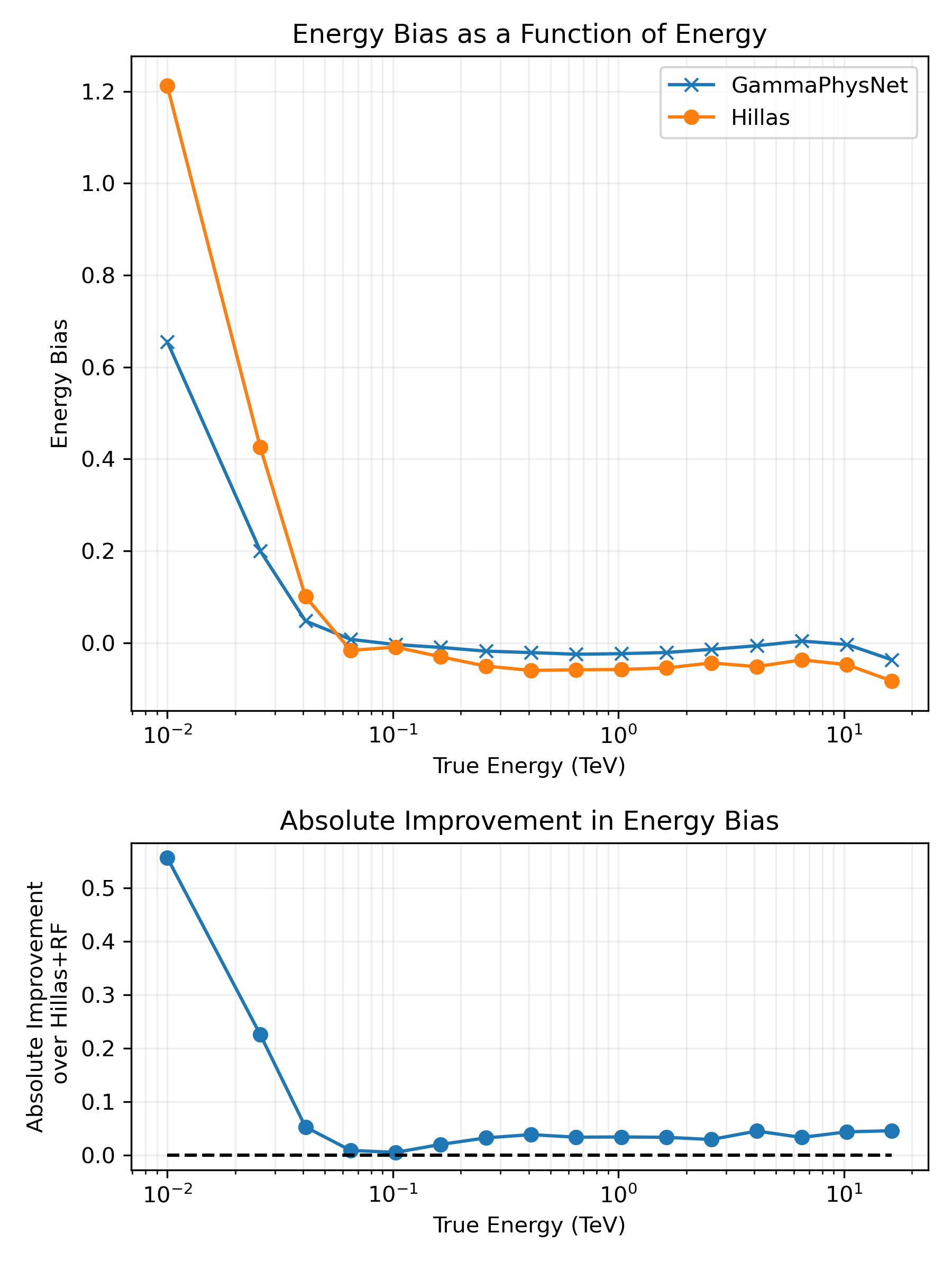
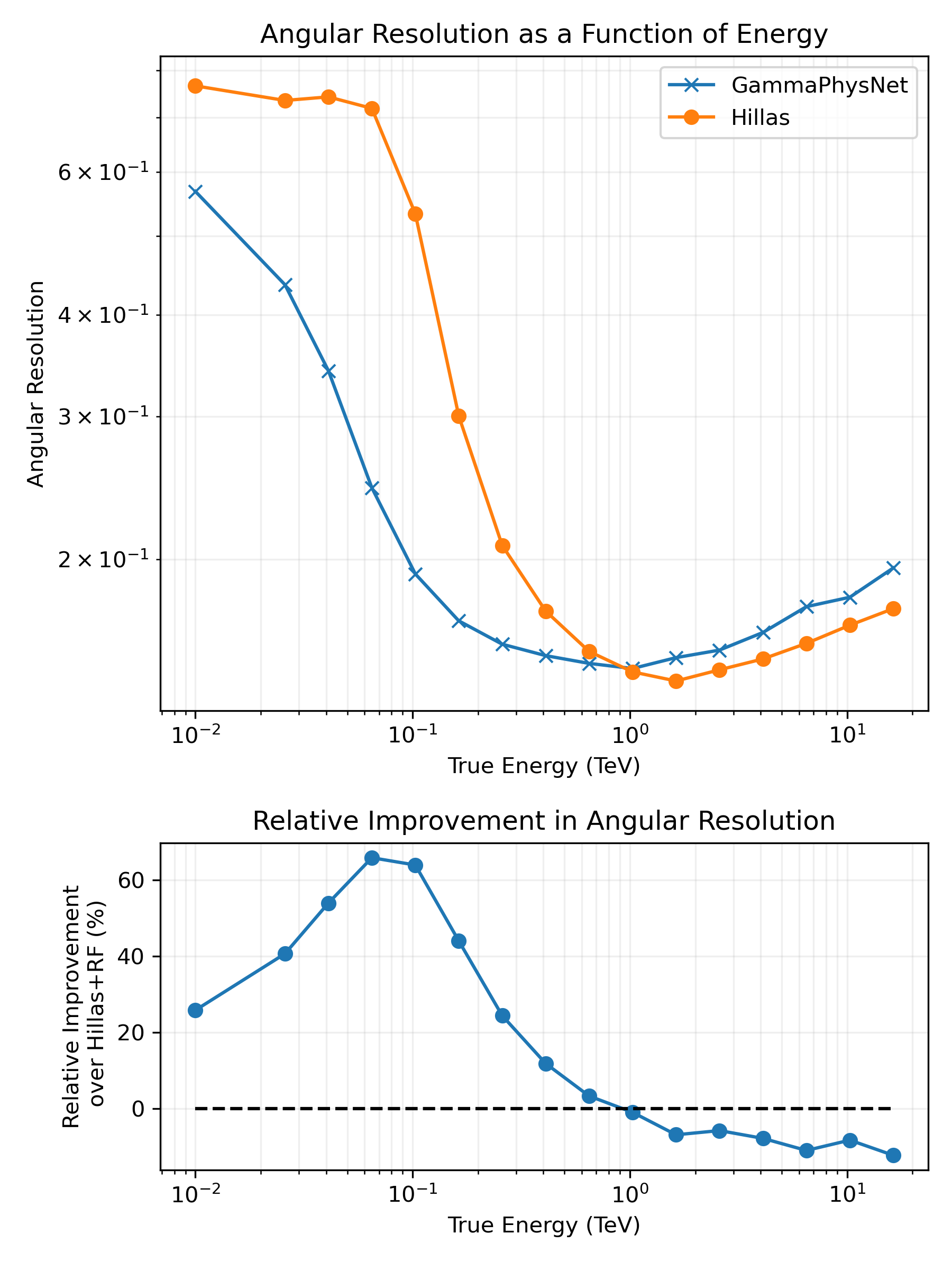
Figures of merit (FOM)
**Model performance evaluation**
| Model output | FOM simulations (labelled) | FOM real data (unlabelled) |
|---|---|---|
| Energy | Energy resolution Energy bias |
- |
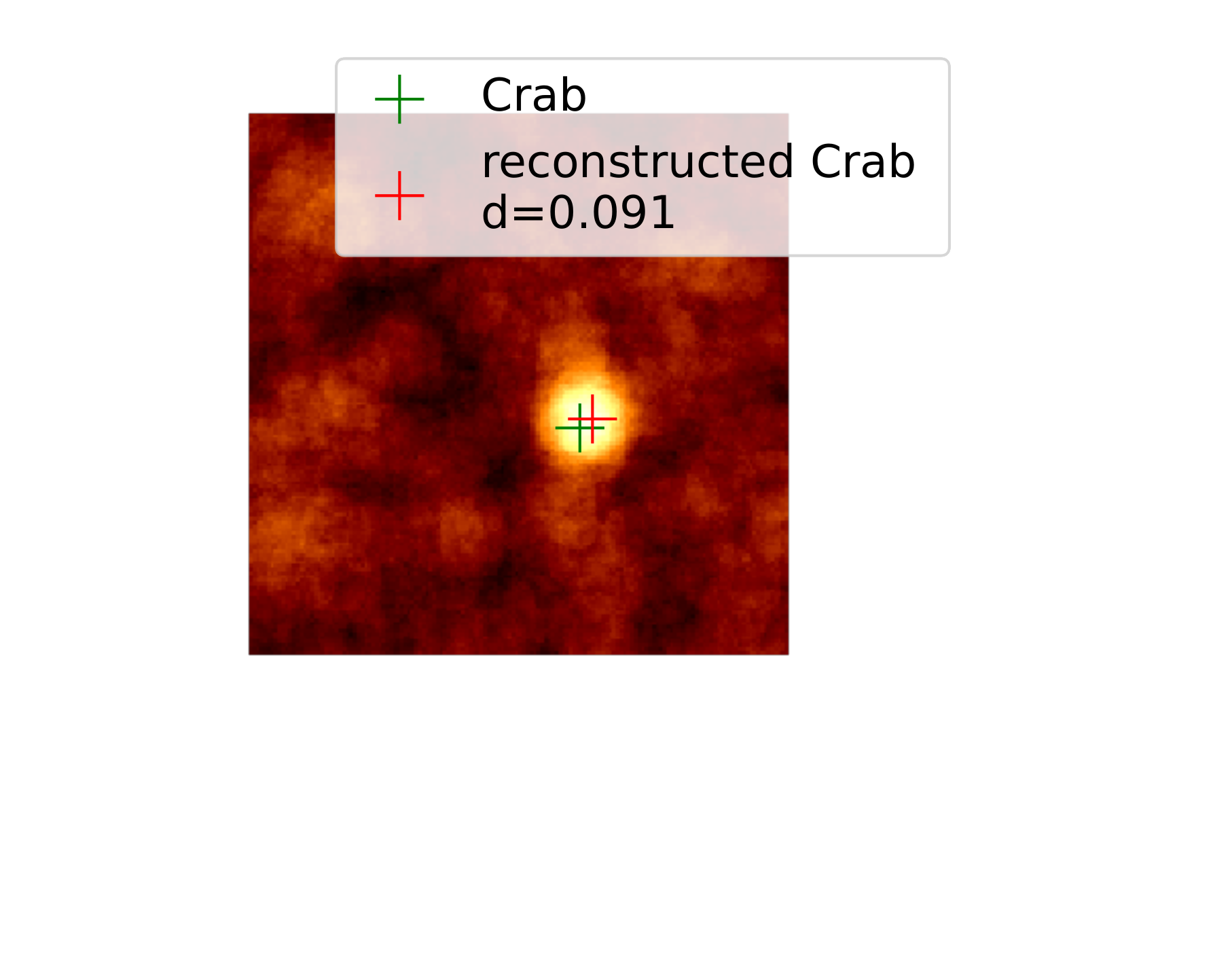
| Direction | Angular resolution | Angular resolution (point source) Reconstruction bias |
| Classification | AUC | Significance |
* Computed per bin of energy * Multiple seeds (initialisation, shuffle) for variability when possible
Presentation outline
- The reconstruction procedure
- Challenging transition from simulations to real observations
- Information fusion
- Domain adaptation
- Transformers
- Conclusion and perspectives
The reconstruction procedure
Discrimination patterns
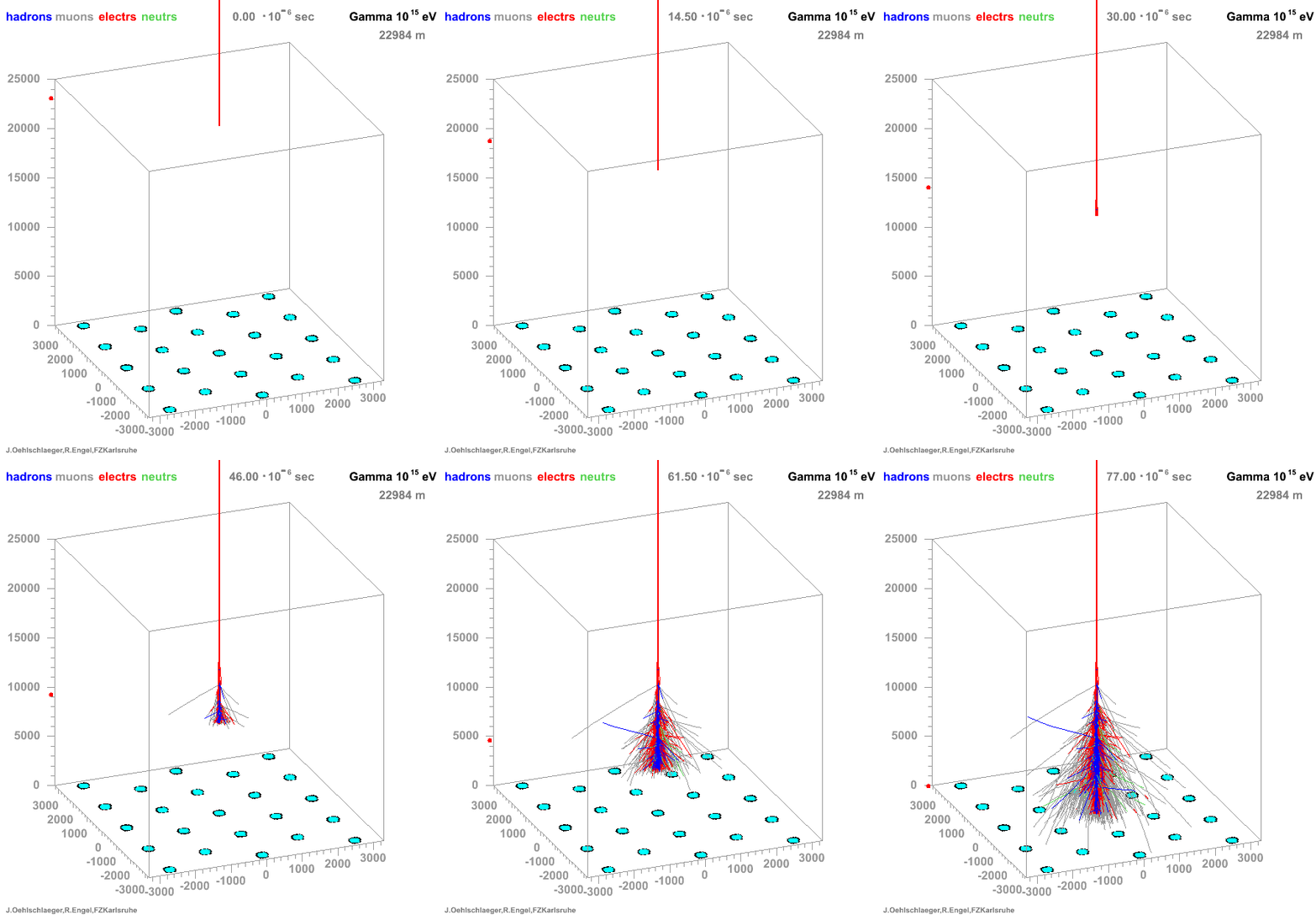
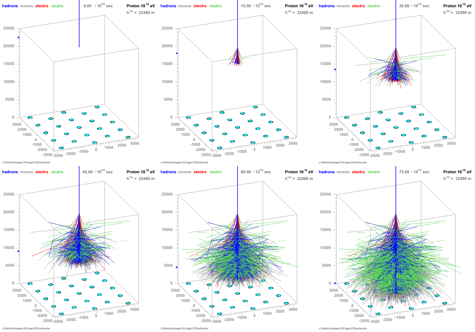
→ Different Cherenkov light emission patterns make distinction possible in acquired images
https://www.iap.kit.edu/corsika/71.php

Standard approaches
Hillas+Random Forest (RF)
* Morphological prior hypothesis: ellipsoidal integrated signal * Uses Hillas parameters (moments) * Leverages multiple RFs * Pros * Fast and robust * Cons * Necessitates image cleaning * Limited at lower energy levels * In production on LST-1 (baseline)
A. M. Hillas. [Cerenkov Light Images of EAS Produced by Primary Gamma Rays and by Nuclei.](https://ntrs.nasa.gov/api/citations/19850026666/downloads/19850026666.pdf) In: 19th International Cosmic Ray Conference (ICRC19), Volume 3. Vol. 3. International Cosmic Ray Conference. Aug. 1985, p. 445. H. Abe et al. [Observations of the Crab Nebula and Pulsar with the Large-sized Telescope Prototype of the Cherenkov Telescope Array](https://arxiv.org/abs/2306.12960) In: Astrophys. J. 956.2 (2023), p. 80
ImPACT and Model++
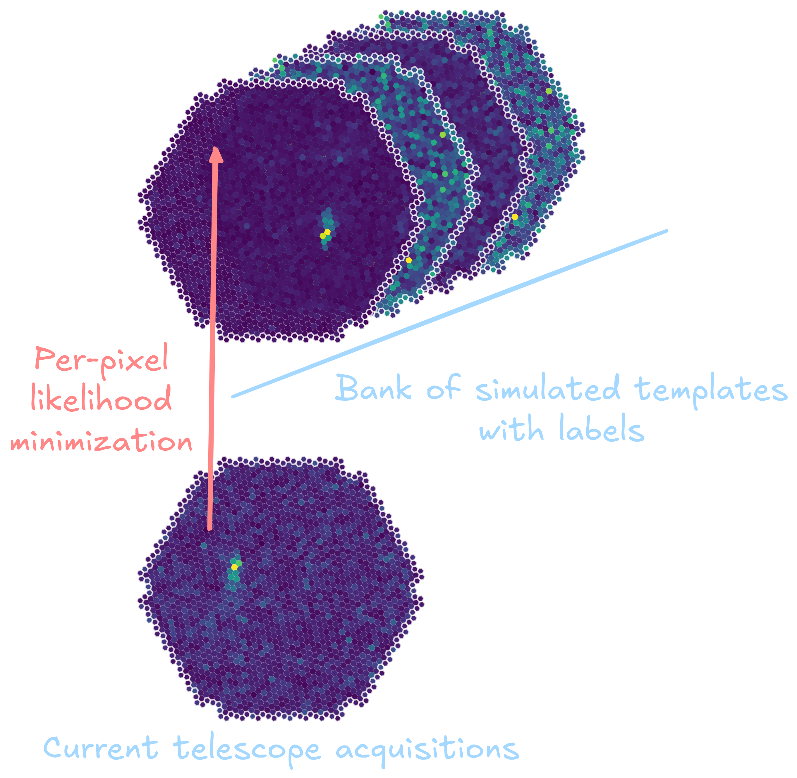
* Simulation of templates * Matching templates to real data using per-pixel likelihood * Background rejection using Boosted Decision Tree on discriminant parameters * Pros * Best overall performance * Cons * Computationally expensive
R.D. Parsons and J.A. Hinton. [A Monte Carlo template based analysis for airCherenkov arrays.](https://arxiv.org/abs/0907.2610) In: Astroparticle Physics 56 (Apr. 2014), pp. 26–34 Mathieu de Naurois and Loïc Rolland. [A high performance likelihood reconstruction of gamma-rays for imaging atmospheric Cherenkov telescopes](https://arxiv.org/abs/0907.2610). In: Astroparticle Physics 32.5 (Dec. 2009), pp. 231–252.
FreePACT
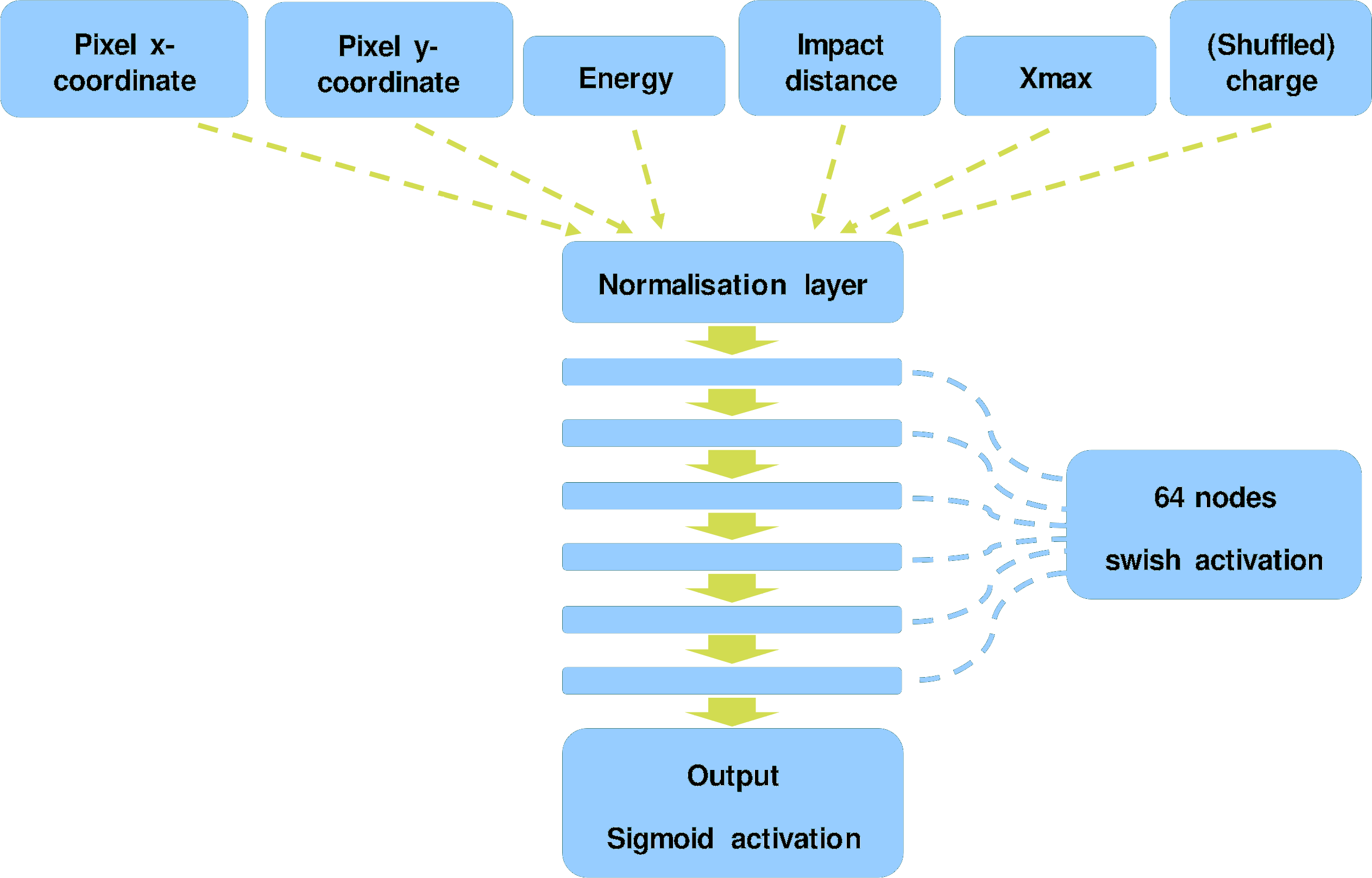
* Neural network to estimate the likelihood-to-evidence ratio * Training the neural network (classifier trained to differentiate between samples drawn from the joint PDF and from the product of the marginal) * Pros * Faster than ImPACT * Yields similar or improved results
Georg Schwefer, Robert Parsons, and Jim Hinton. [A Hybrid Approach to Event Reconstruction for Atmospheric Cherenkov Telescopes Combining Machine Learning and Likelihood Fitting.](https://arxiv.org/abs/2406.17502) 2024
$\gamma$-PhysNet
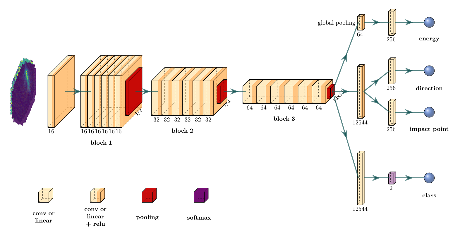
* CNN-based (interpolated inputs) * Backbone with dual attention * Multi-task architecture * Pros * No prior hypothesis * Less preprocessing (e.g. no cleaning) * Cons * Tricky to optimize * Black-box nature * Expectations * Performance $\geq$ ImPACT / FreePACT * Fast inference
A. Demichev and A. Kryukov. [Using deep learning methods for IACT data analysis in gamma-ray astronomy: A review](https://www.sciencedirect.com/science/article/pii/S2213133724000088) 2024. Mikaël Jacquemont. [Cherenkov Image Analysis with Deep Multi-Task Learning from Single-Telescope Data.](https://hal.archives-ouvertes.fr/hal-03043188) Theses. Université Savoie Mont Blanc, Nov. 2020.
* Real labelled data are intrinsically unobtainable * Training relying on simulations * Simulations are approximations of the reality
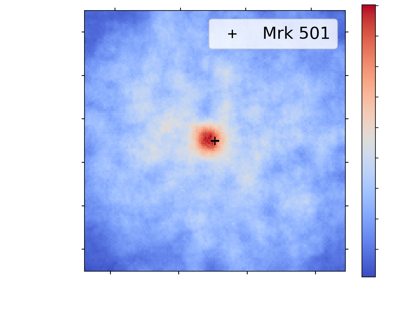
| Reconstruction algorithm | Significance (higher is better) | Excess of $\gamma$ | Background count |
|---|---|---|---|
| $\gamma$-PhysNet | 12.5 σ | 395 | 302 |
| $\gamma$-PhysNet + Background matching | 14.3 σ | 476 | 317 |
Tab. Detection capability of the $\gamma$-PhysNet on Crab observations
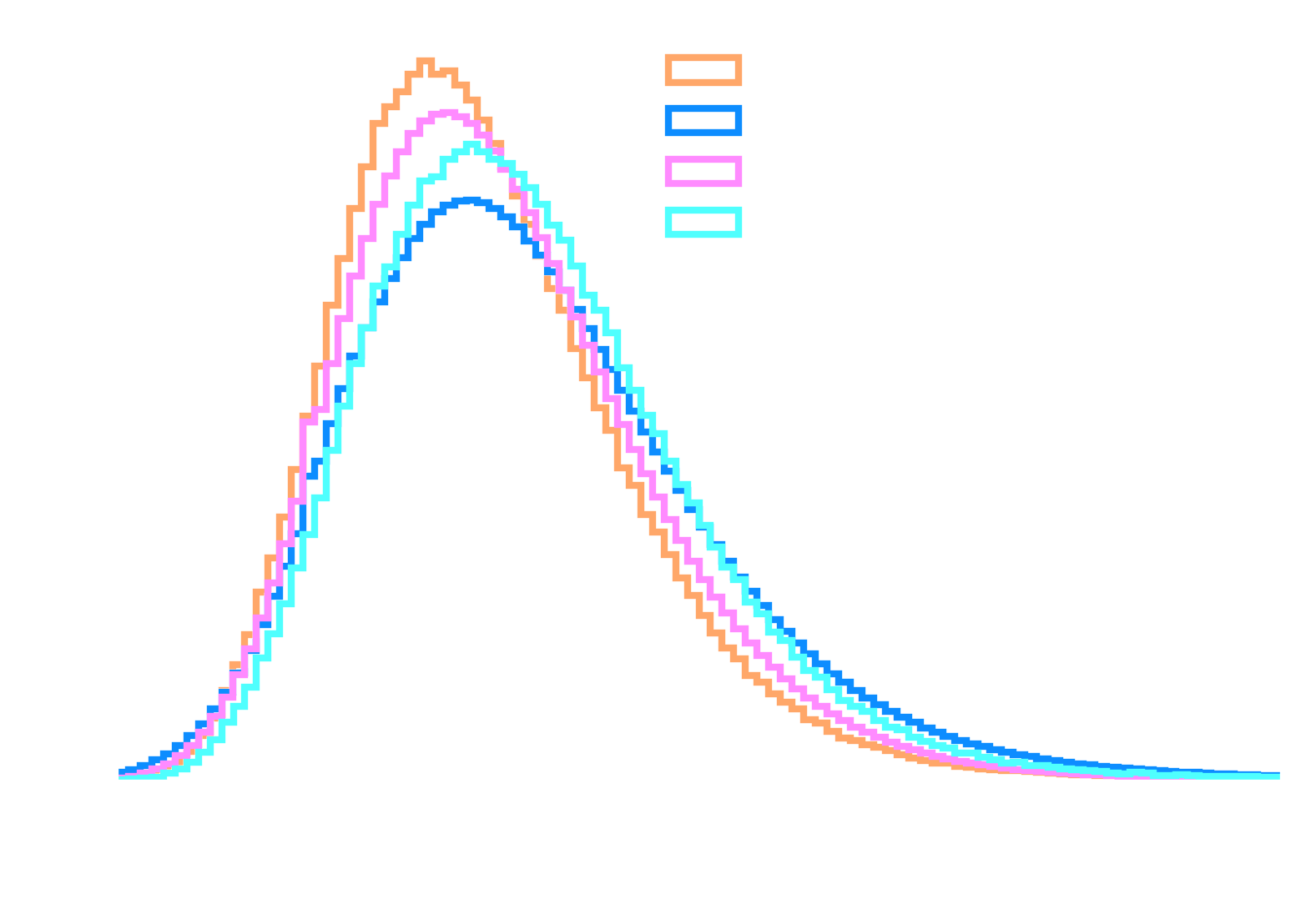
- Data adaptation is limited to NSB variations
- Poisson approximation
- Pixel independence
Thomas Vuillaume et al. [Analysis of the Cherenkov Telescope Array first LargeSized Telescope real data using convolutional neural networks](https://arxiv.org/abs/2108.04130.pdf) 2021
Challenging transition from simulations to real observations
(thesis contribution)Quantifiable differences
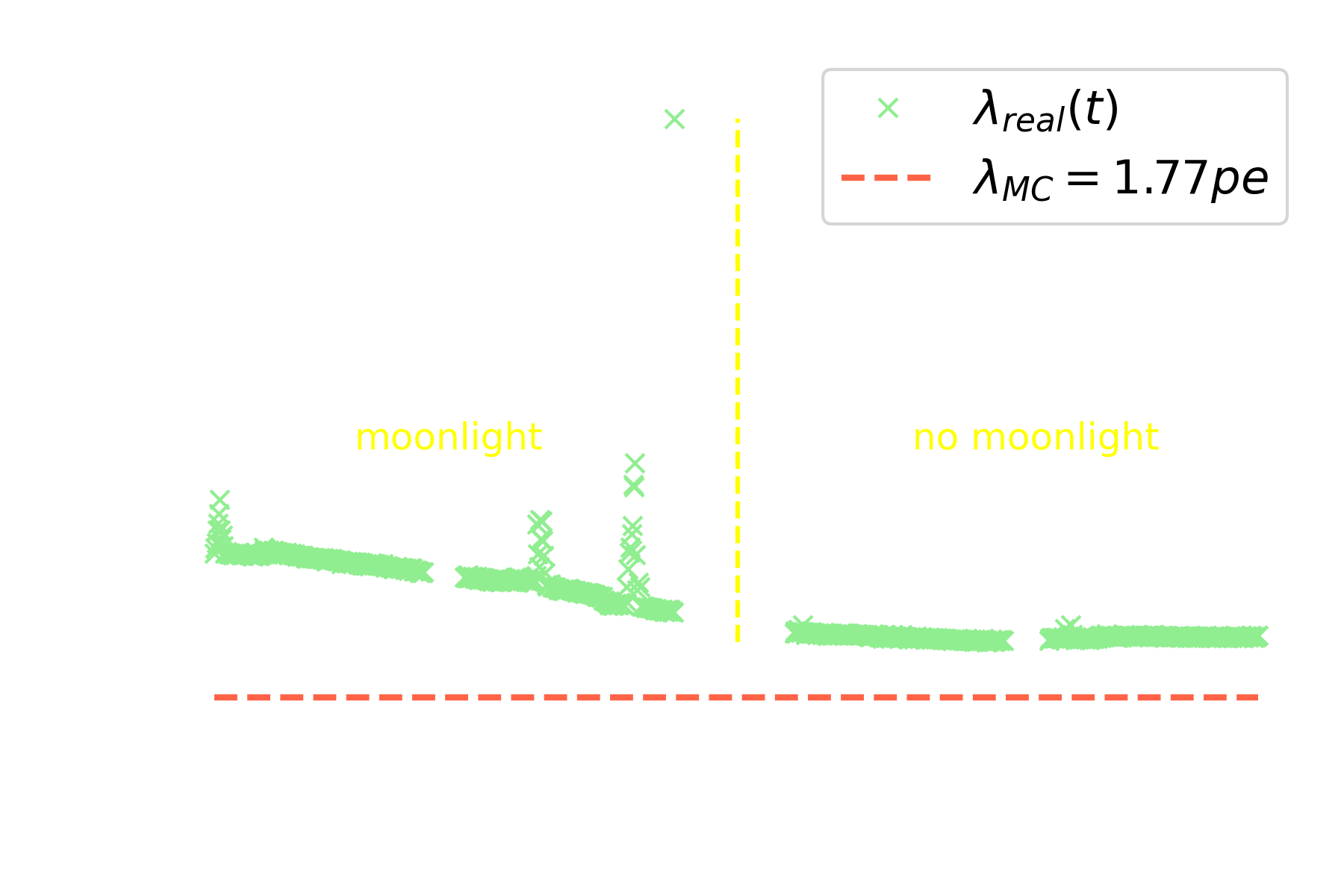
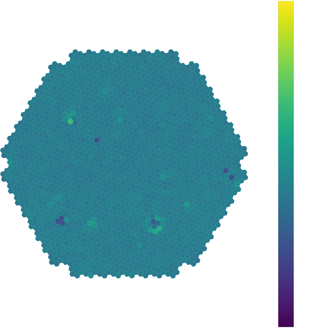
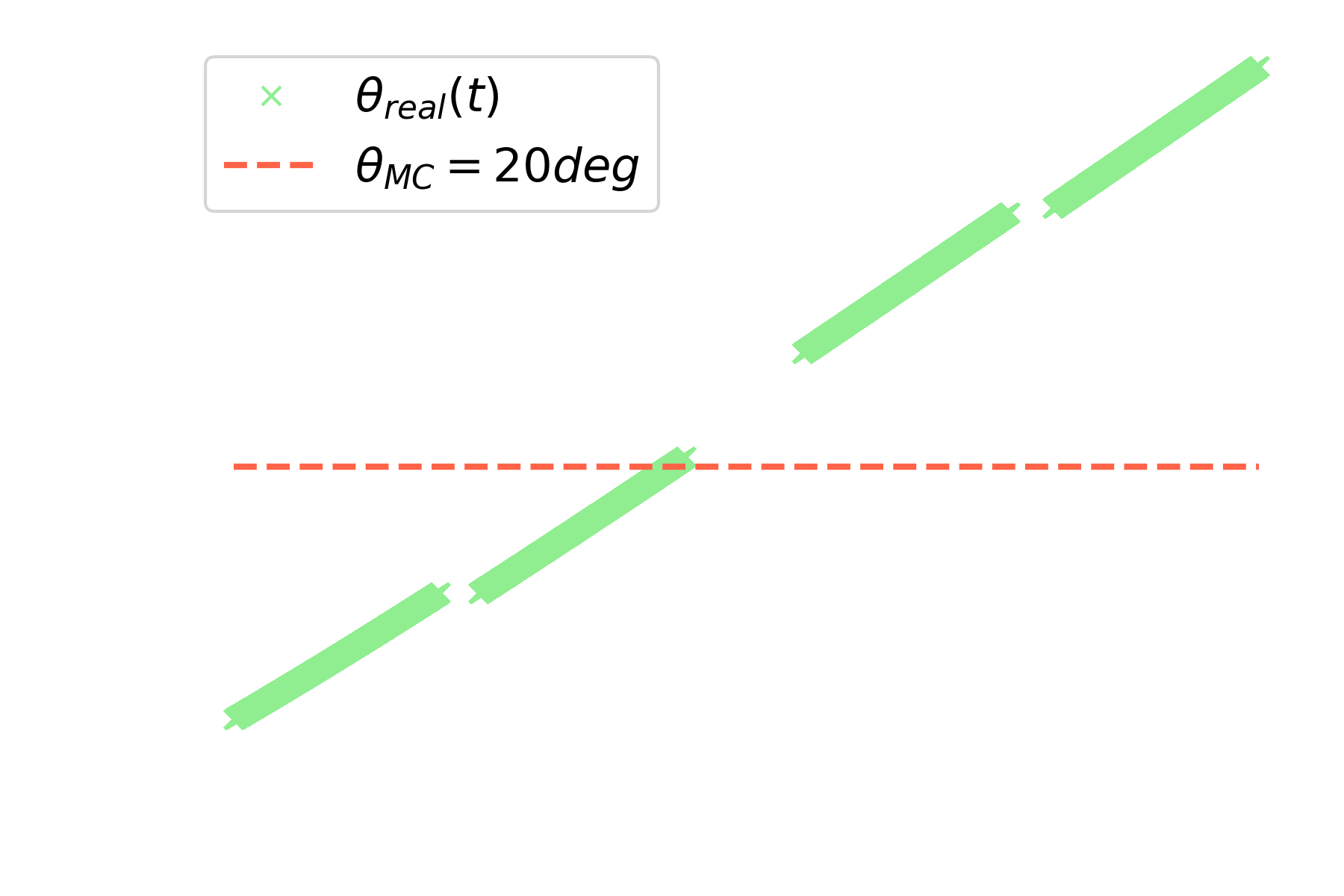
* Training simulations are not available at all pointing directions * More atmosphere traversed at higher zenith angles → More absorption and scattering
| Run number | 6892 | 6893 | 6894 | 6895 |
|---|---|---|---|---|
| Avg. $\theta_{real}$ (deg) | 14.0 | 18.1 | 25.7 | 30.2 |
| Avg. $\lambda_{real}$ (pe) | 2.46 | 2.35 | 2.07 | 2.07 |
| $\delta \theta = \theta_{real} - \theta_{MC}$ (deg) | -7.0 | -1.9 | 5.7 | 10.2 |
| $\delta \lambda = \lambda_{real} - \lambda_{MC}$ (pe) | 0.70 | 0.59 | 0.31 | 0.31 |
* More quantifiable differences (fog in camera, clouds, calima, etc) * Unknown and unquantifiable differences also exist * Data adaptation (background matching) is not sufficient
R. D. Parsons, A. M. W. Mitchell, and S. Ohm. [Investigations of the Systematic Uncertainties in Convolutional Neural Network Based Analysis of Atmospheric Cherenkov Telescope Data.](https://arxiv.org/abs/2203.05315) 2022
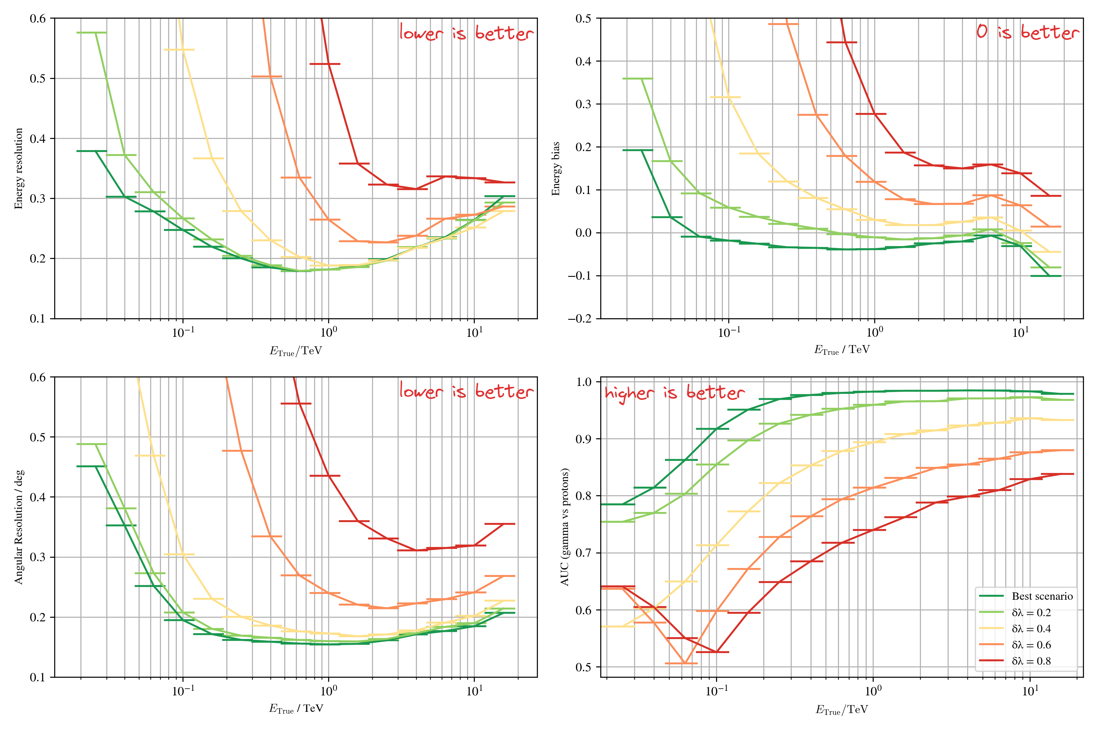
Impact of NSB on the $\gamma$-PhysNet
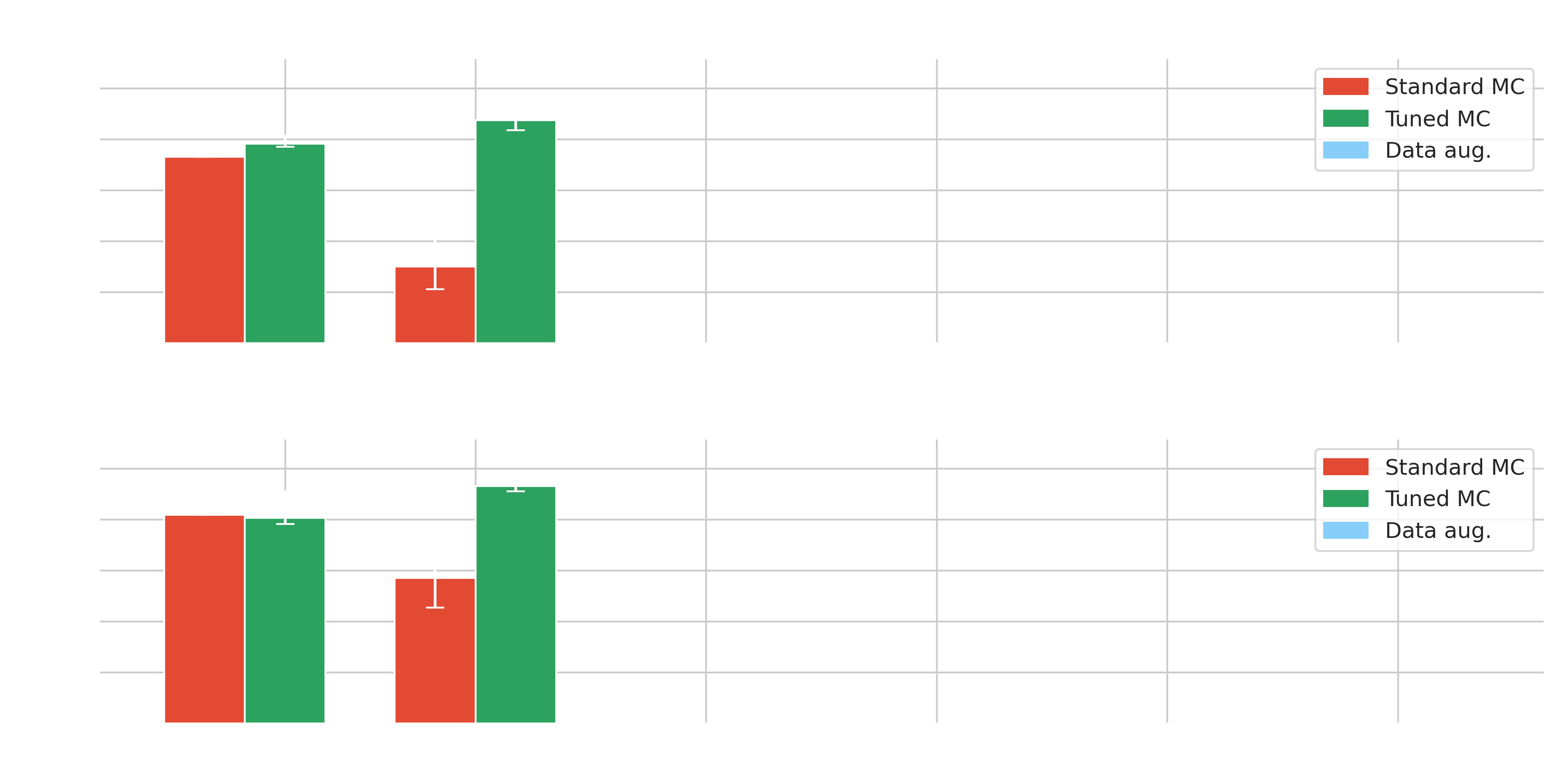
Results on Crab - Baseline




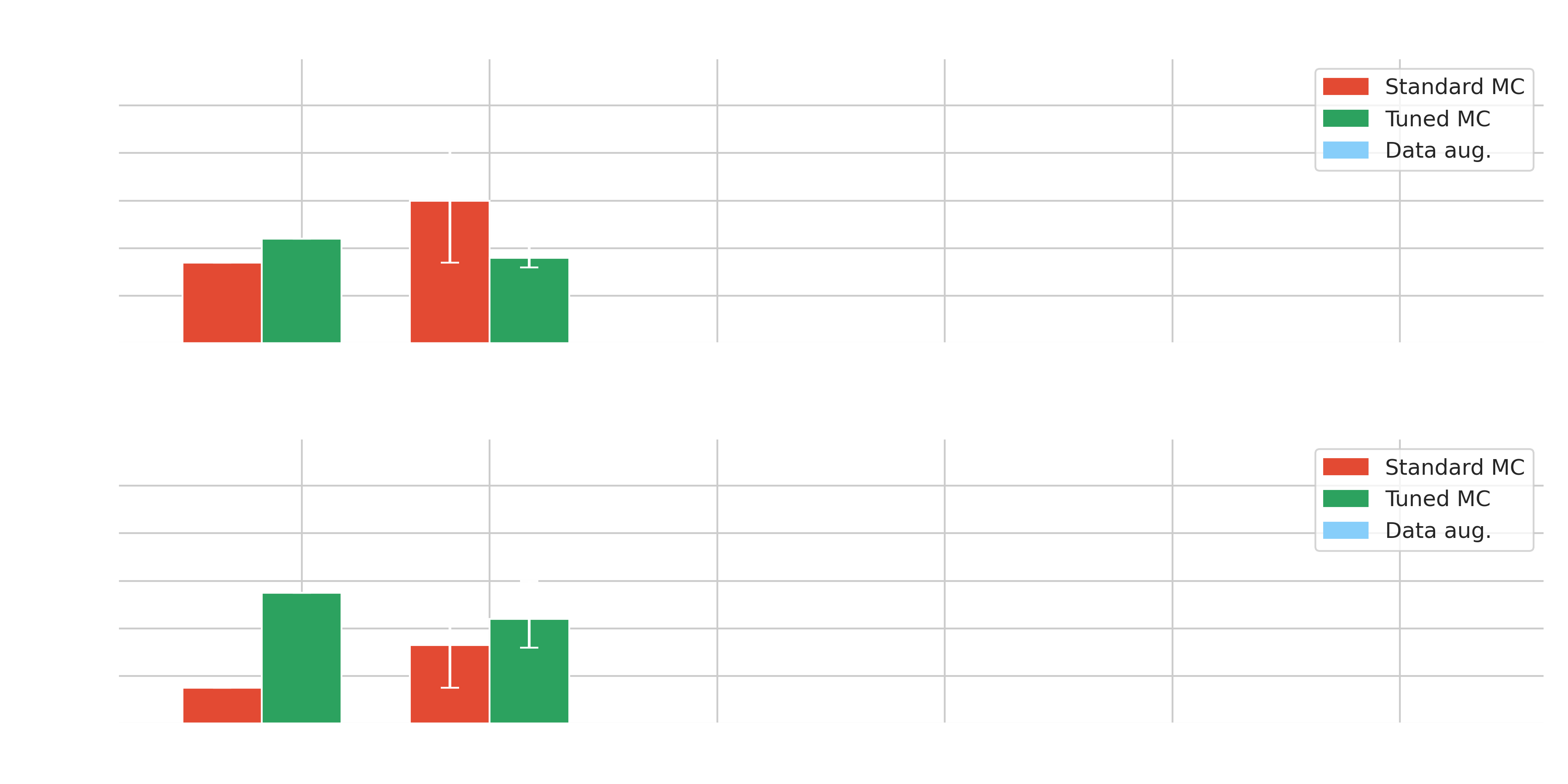


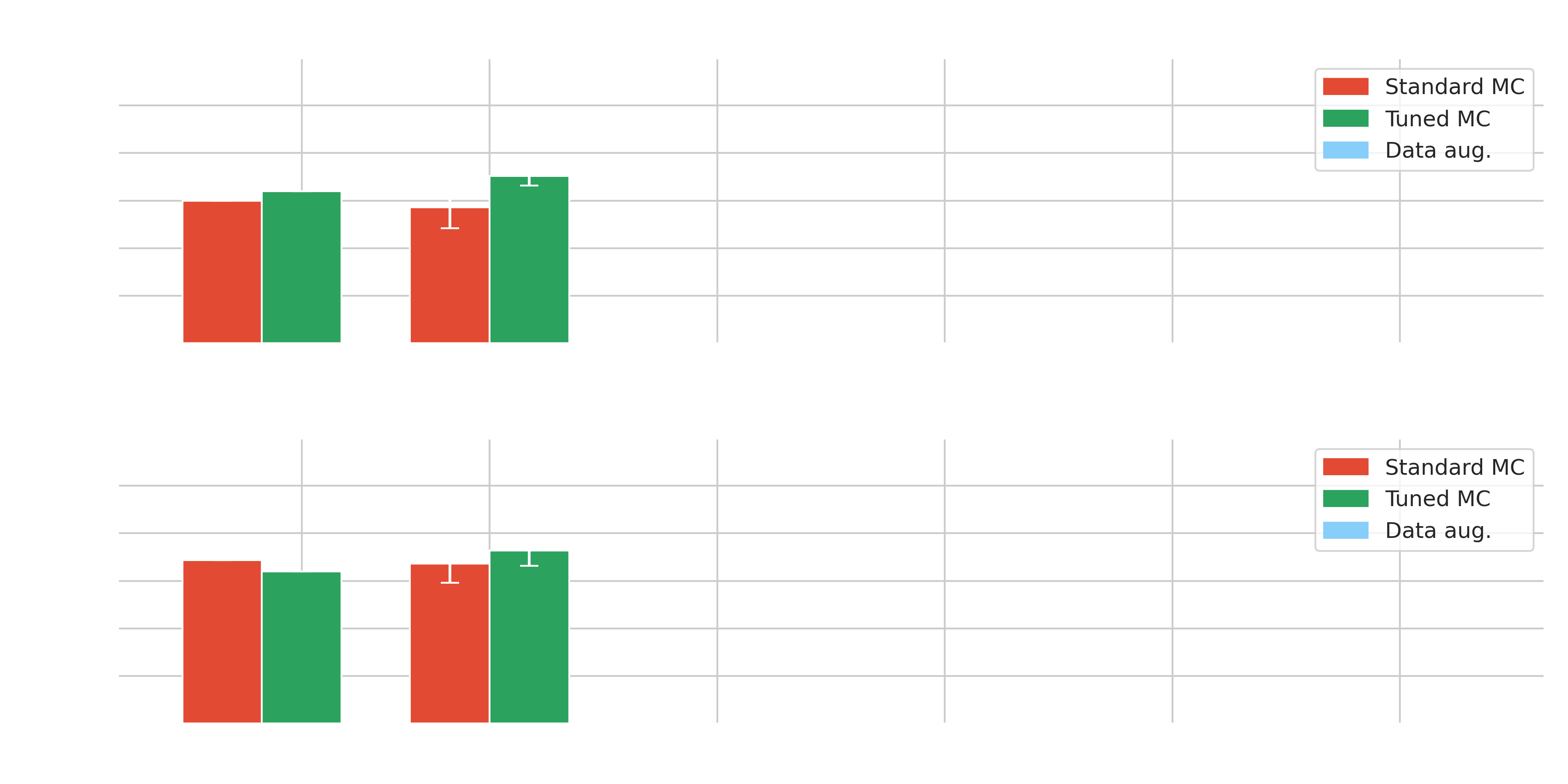
Research direction
**Don't change the data, change the model**
Inject NSB information into the model
Information fusion
Make the model agnostic to changes
Domain adaptation
Improve generalization with pre-training
Transformers
Information fusion
(thesis contribution)Information fusion
Normalization (pre-GPU era) * Trick to stabilize and accelerate the speed of convergence * Maintains stable gradients * Diminishes initialization influence * Allows greater learning rates → Batch Normalization (2015)
\[ O_{i,c,x,y} = \gamma_c \dfrac{F_{i,c,x,y} - \mu_c}{\sqrt{\sigma_c + \epsilon}} + \beta_c \]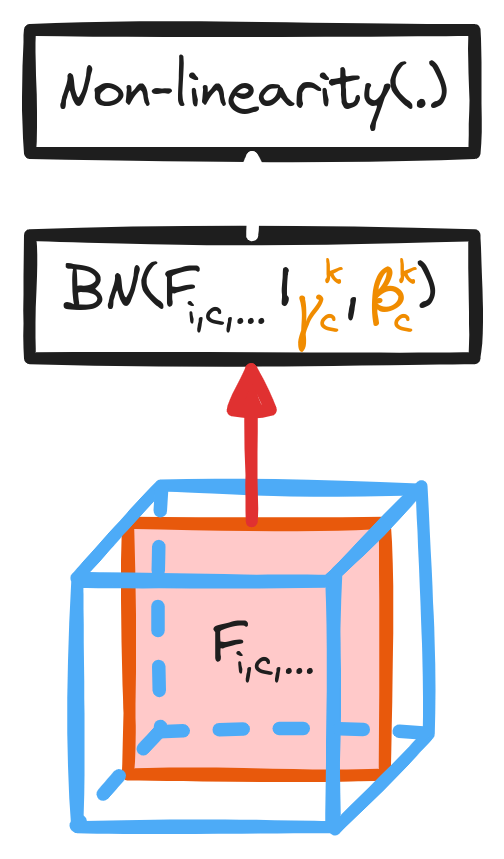
Yann A. LeCun et al. [Efficient BackProp](https://link.springer.com/chapter/10.1007/978-3-642-35289-8_3). In: Neural Networks: Tricks of the Trade: Second Edition. Ed. by Grégoire Montavon, Geneviève B. Orr, and Klaus Robert Müller. Berlin, Heidelberg: Springer Berlin Heidelberg, 2012, pp. 9–48 Sergey Ioffe and Christian Szegedy. [Batch Normalization: Accelerating Deep Network Training by Reducing Internal Covariate Shift.](https://arxiv.org/abs/1502.03167) 2015
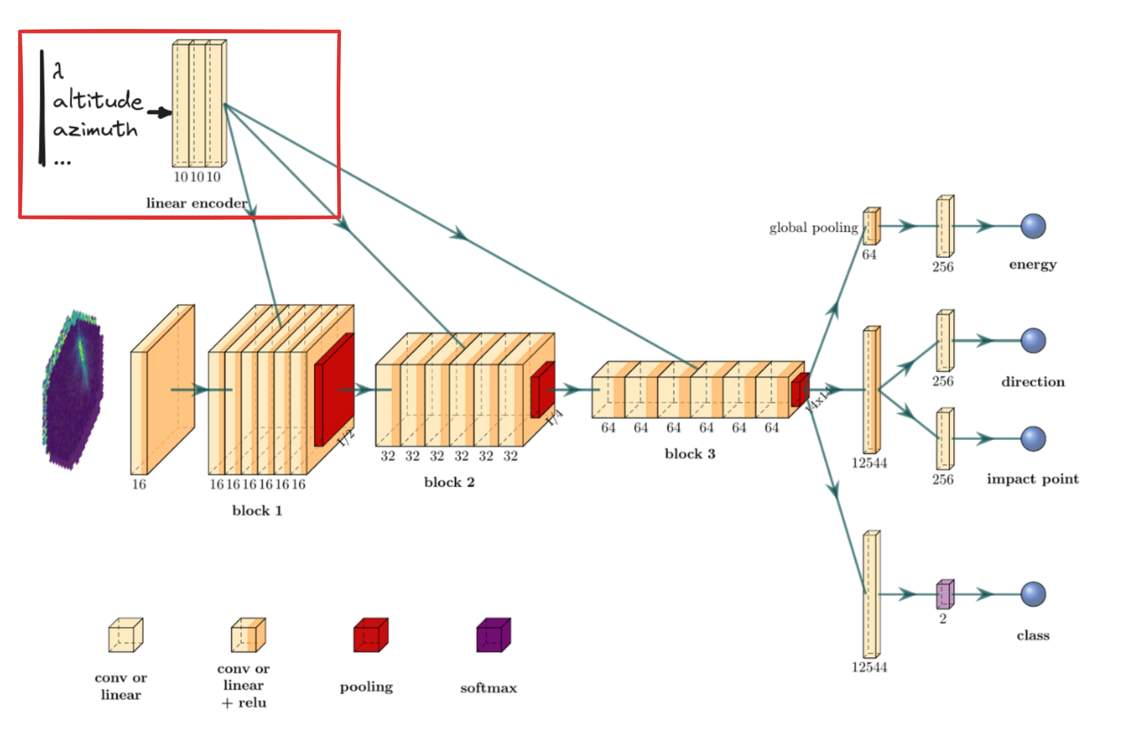
Conditional Batch Normalization (2017) * Elegant way to inject additional information within the network * NSB and pointing direction affects the distributions of the input data
\[ O_{i,c,x,y} = (\gamma_c + \Delta \gamma_c) \dfrac{F_{i,c,x,y} - \mu_c}{\sqrt{\sigma_c + \epsilon}} + (\beta_c + \Delta \beta_c) \]→ Used with data augmentation
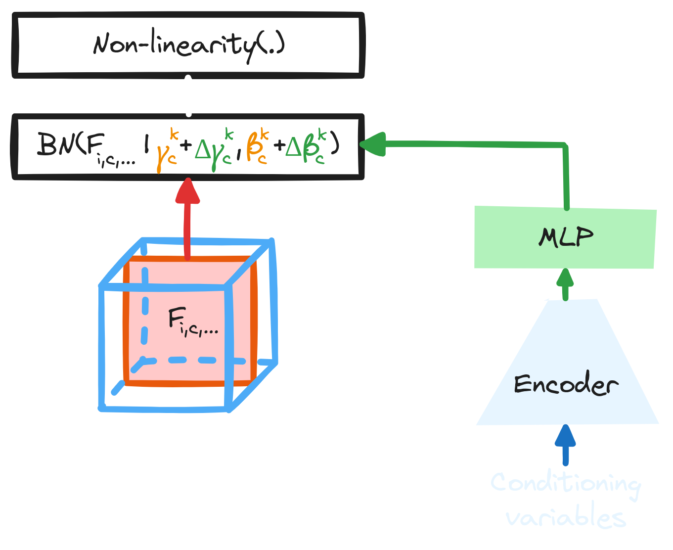
Harm de Vries et al. [Modulating early visual processing by language.](https://arxiv.org/abs/1707.00683) 2017
The $\gamma$-PhysNet-CBN architecture
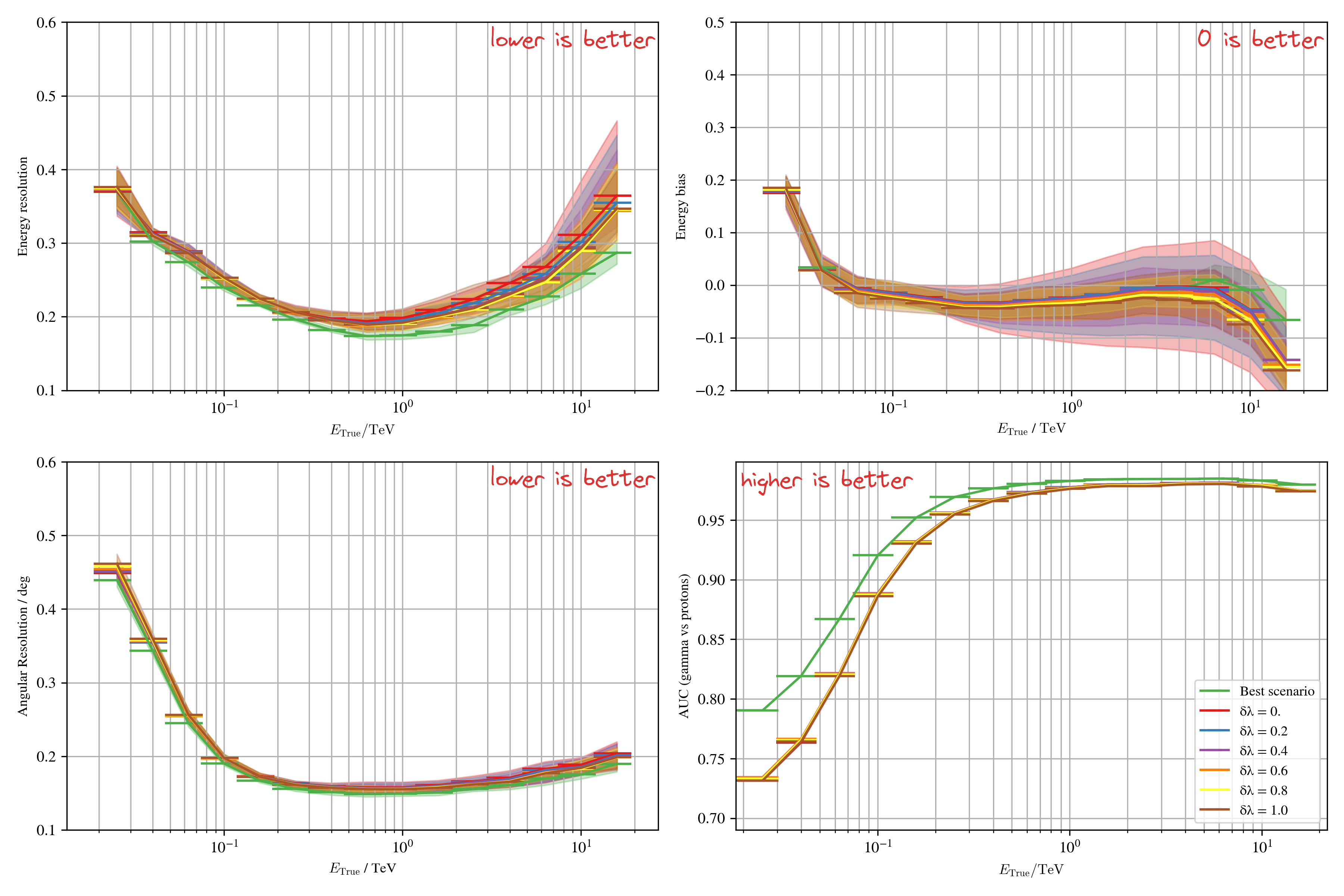
Results with multi-modality on simulations
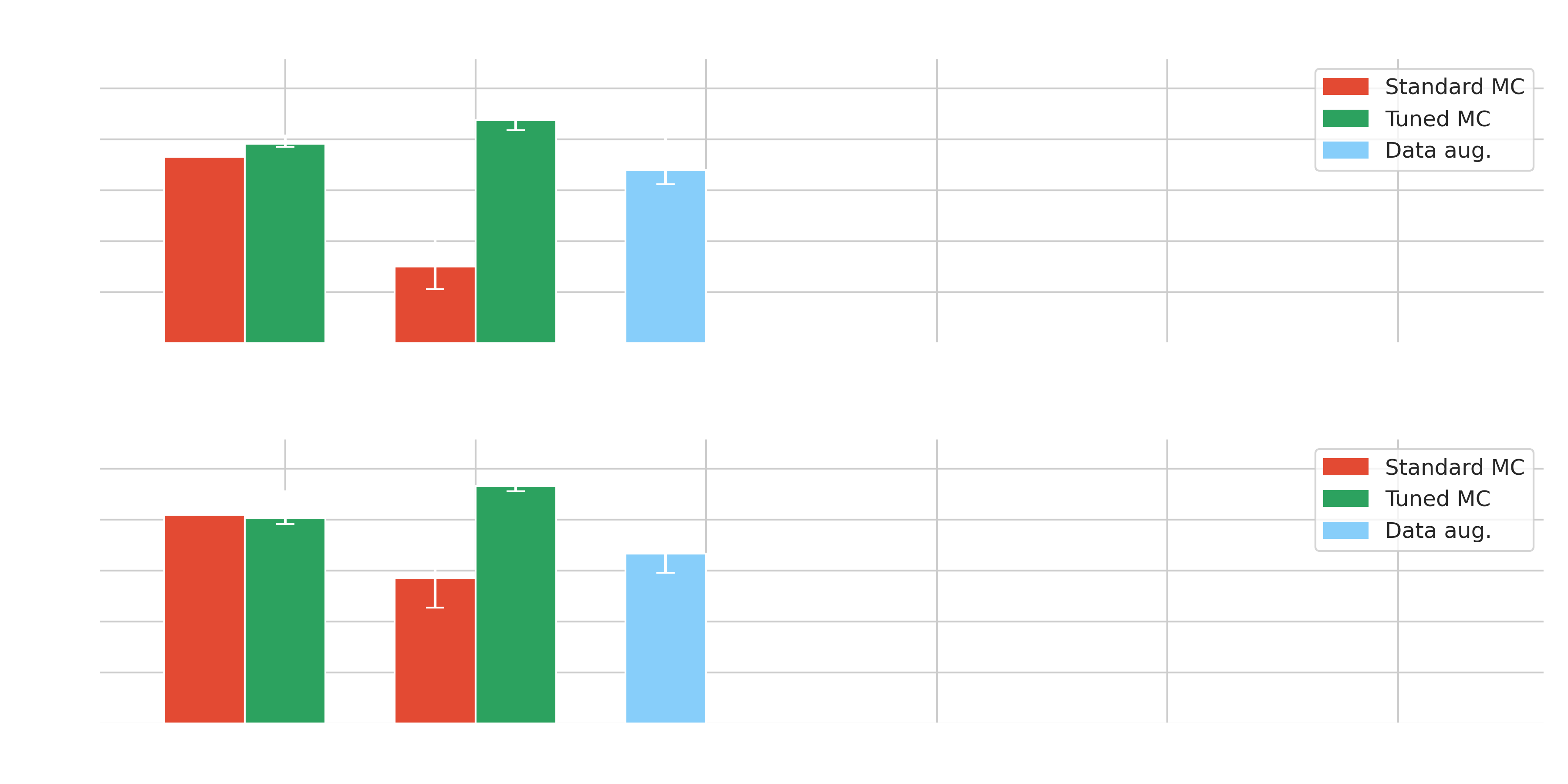
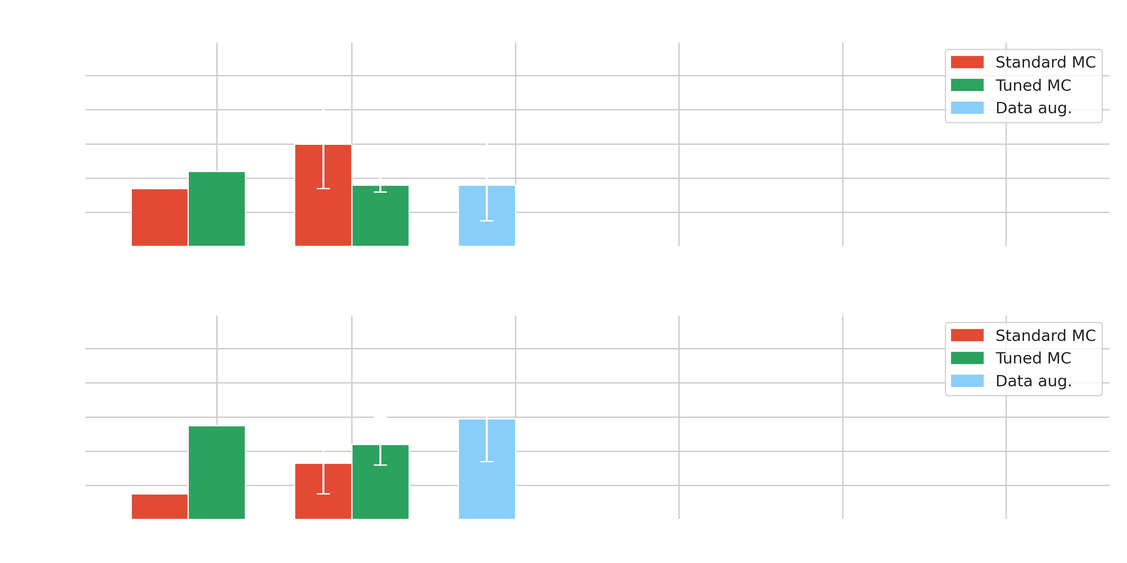
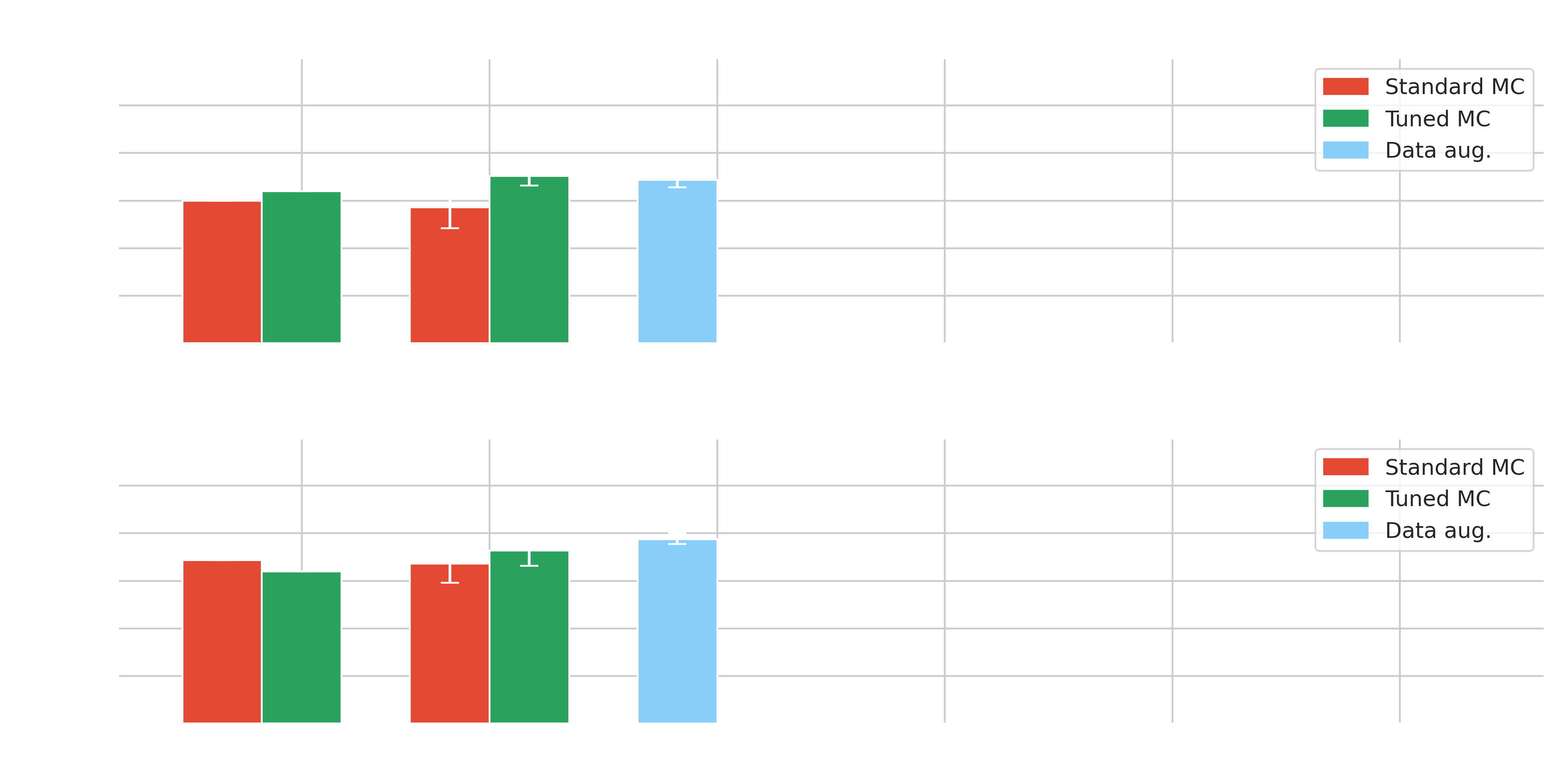
Results on Crab - $\gamma$-PhysNet-CBN






Domain adaptation
(thesis contribution)Unsupervised Domain Adaptation (UDA)
**[Domain adaptation](https://arxiv.org/abs/2009.00155): Set of algorithms and techniques to reduce domain discrepancies**
* Domain $\mathcal{D} = (\mathcal{X}, P(x))$ * Take into account unknown differences between * Source domain (labelled simulations) * Target domain (unlabelled real data) * Include unlabelled real data in the training * No target labels → Unsupervised * Selection and improvement of relevant SOTA: DANN, DeepJDOT, DeepCORAL
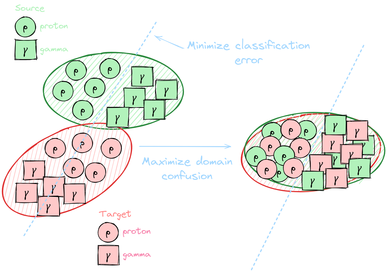
Yaroslav Ganin et al. [Domain-Adversarial Training of Neural Networks.](https://arxiv.org/abs/1505.07818) 2016. Bharath Bhushan Damodaran et al. [DeepJDOT: Deep Joint Distribution Optimal Transport for Unsupervised Domain Adaptation”](https://arxiv.org/abs/1803.10081) 2018. Baochen Sun and Kate Saenko. [Deep CORAL: Correlation Alignment for Deep Domain Adaptation](https://arxiv.org/abs/1607.01719) 2016.
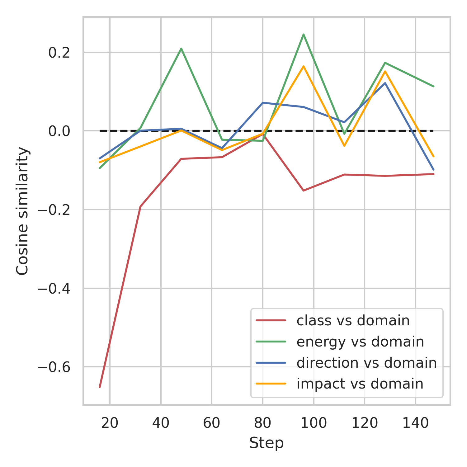
Multi-task balancing
**Multi-task balancing (MTB): Simulateneous optimization of multiple tasks**

* $\neq$ Single-task learning * Correlated tasks help each other to learn better * Conflicting gradients (amplitude and/or direction) * Uncertainty Weighting (UW) → Most performing method for the $\gamma$-PhysNet but limited to MSE, MAE, CE * GradNorm (GN) → More general but tricky to optimize
Sebastian Ruder. [An overview of gradient descent optimization algorithms.](https://arxiv.org/abs/1706.05098) 2017. Alex Kendall et al. [Multi-Task Learning Using Uncertainty to Weigh Losses for Scene Geometry and Semantics.](https://arxiv.org/abs/1705.07115) 2018 Zhao Chen et al. [GradNorm: Gradient Normalization for Adaptive Loss Balancing in Deep Multitask Networks.](https://arxiv.org/abs/1711.02257) 2018
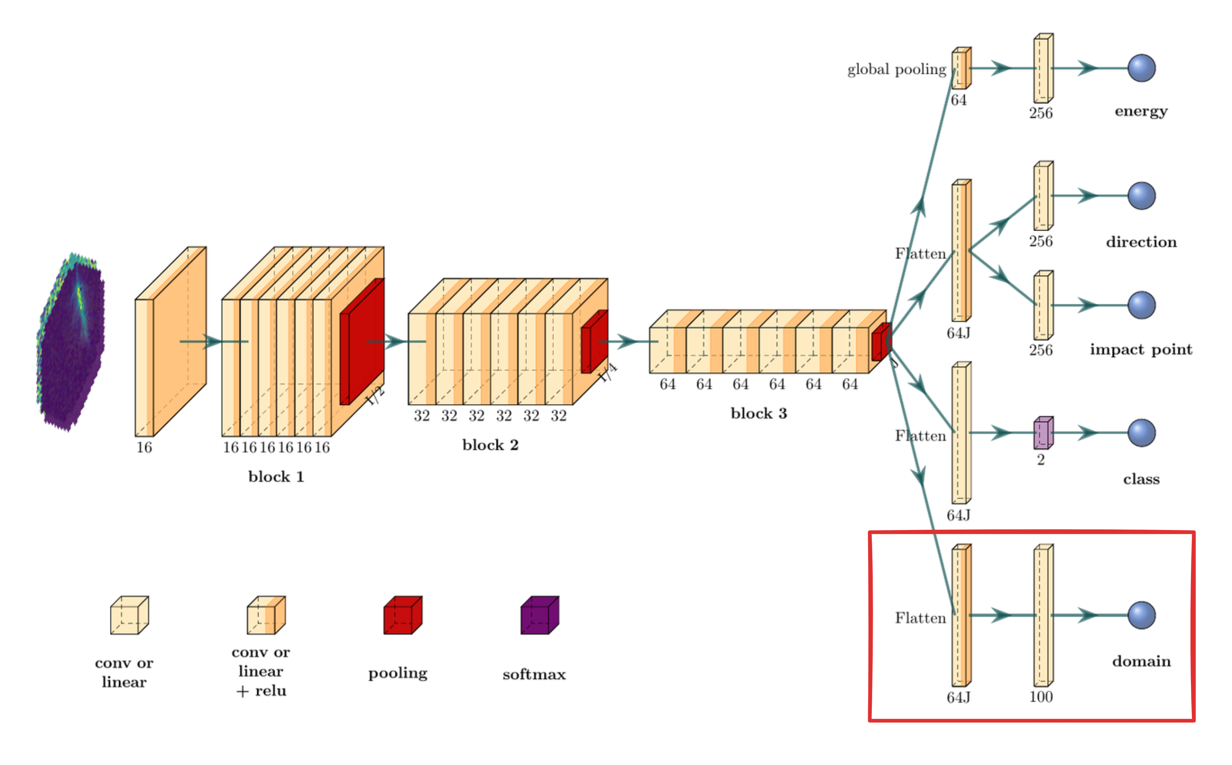
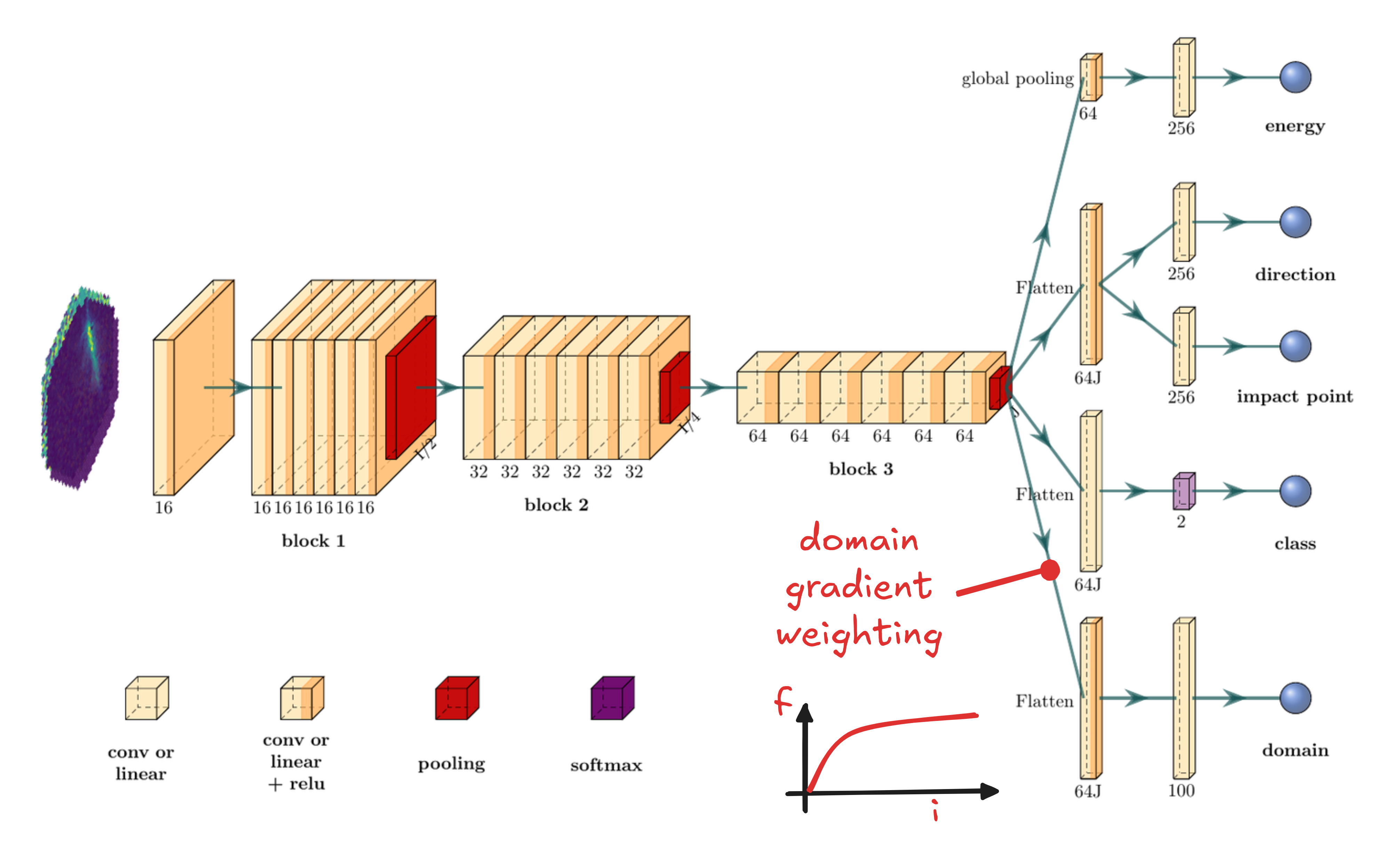
The $\gamma$-PhysNet-DANN architecture
Challenge #1: multi-task optimization
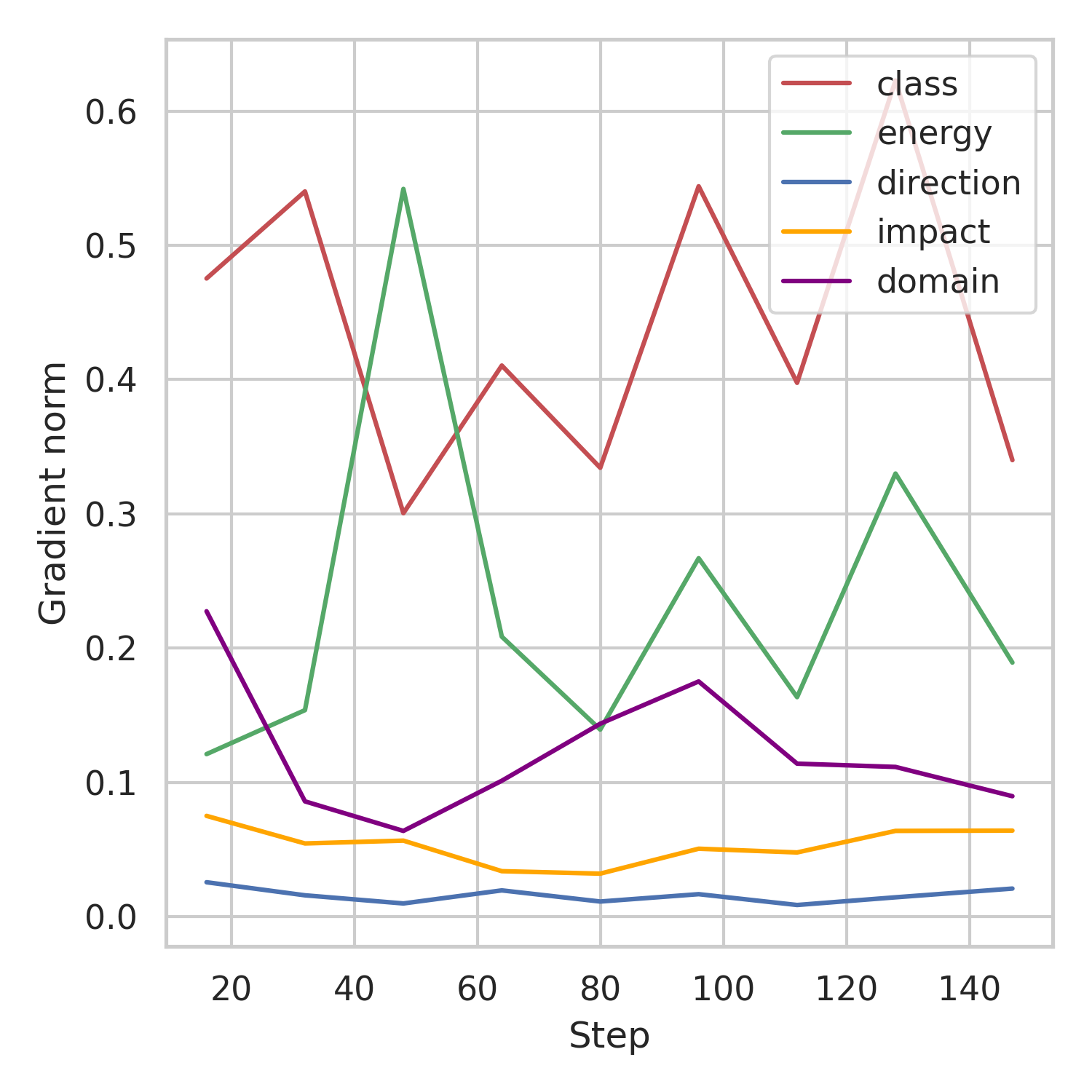
Gradient Layer
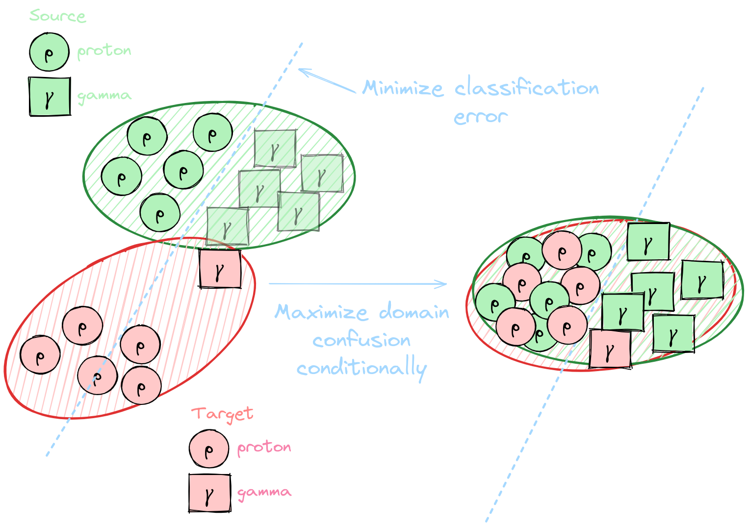
Challenge #2: label shift
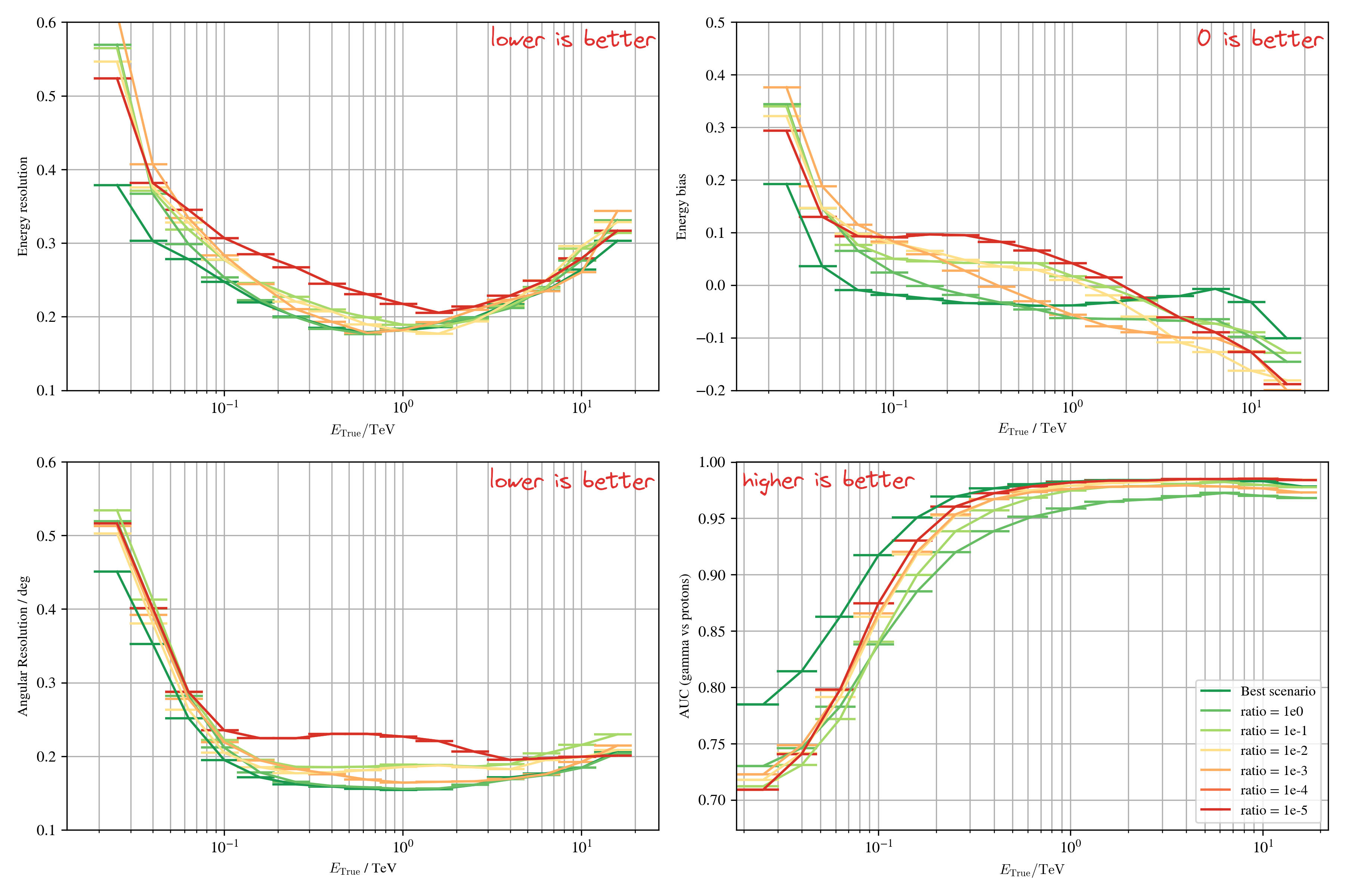
Domain conditioning

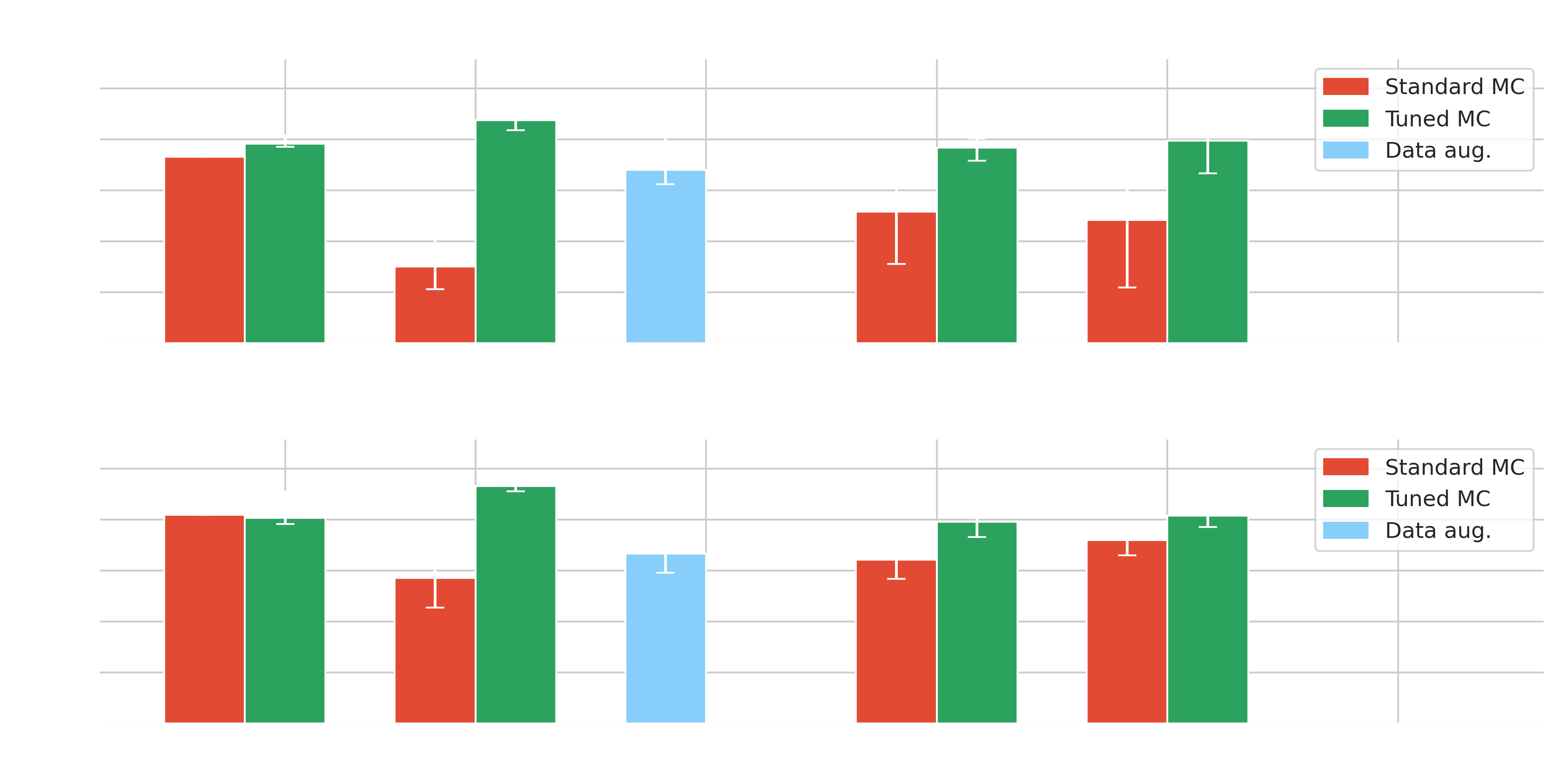
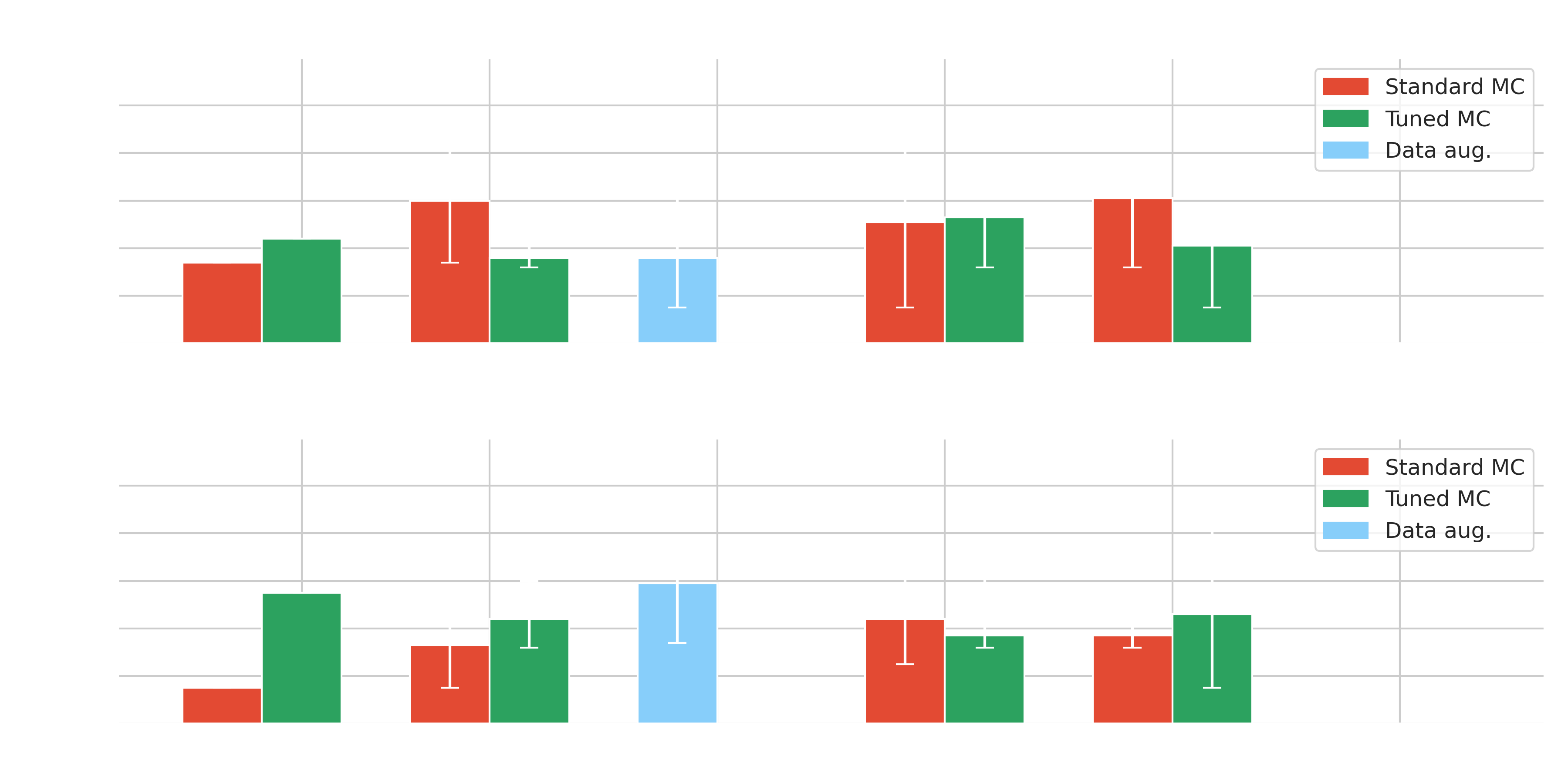
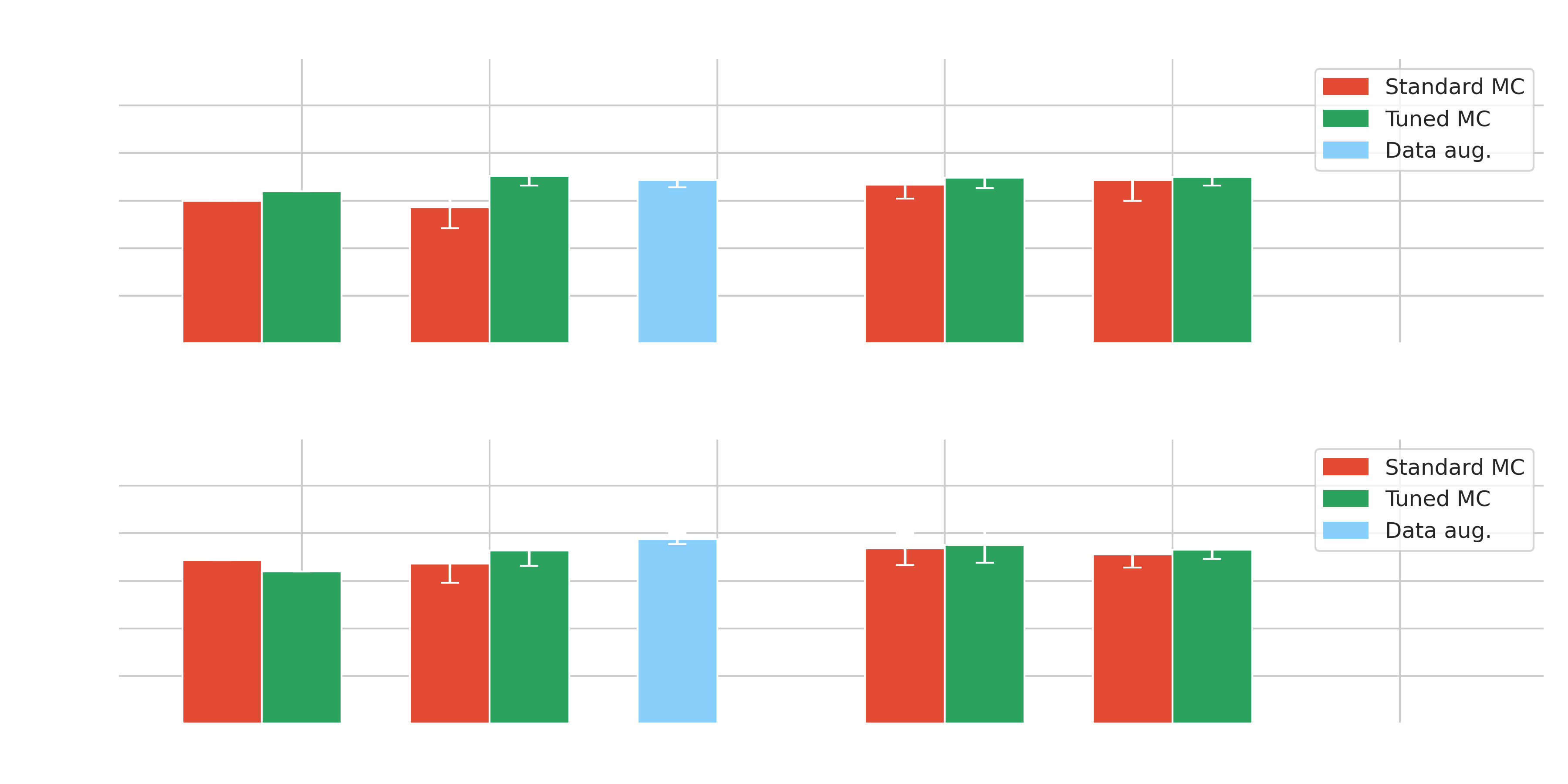
Results on Crab - $\gamma$-PhysNet-(C)DANN






Transformers
(thesis contribution)Transformer models
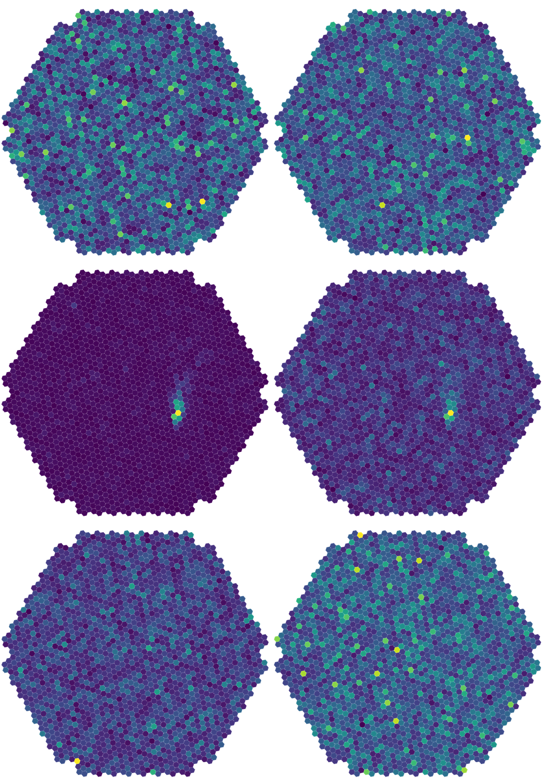
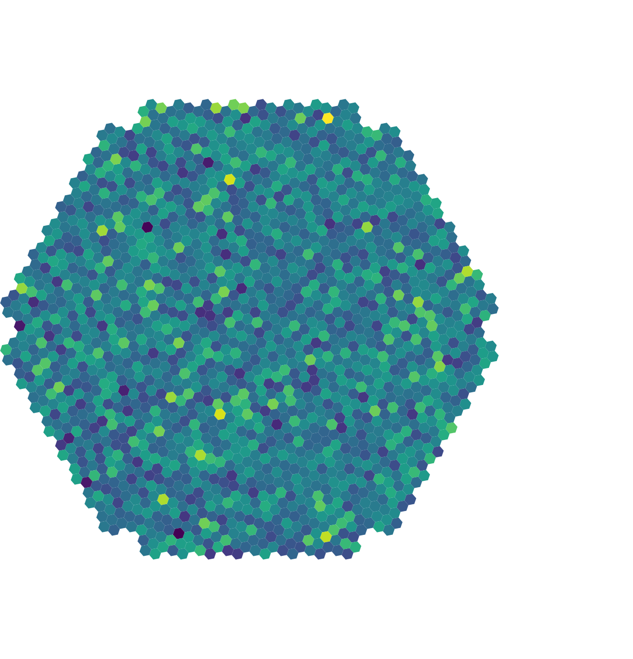
* Image contains redundances * Keep 25% of the patches * In-painting task * Allows to use the hexagonal grid of pixels * Use simulations and real data * Improved generalization
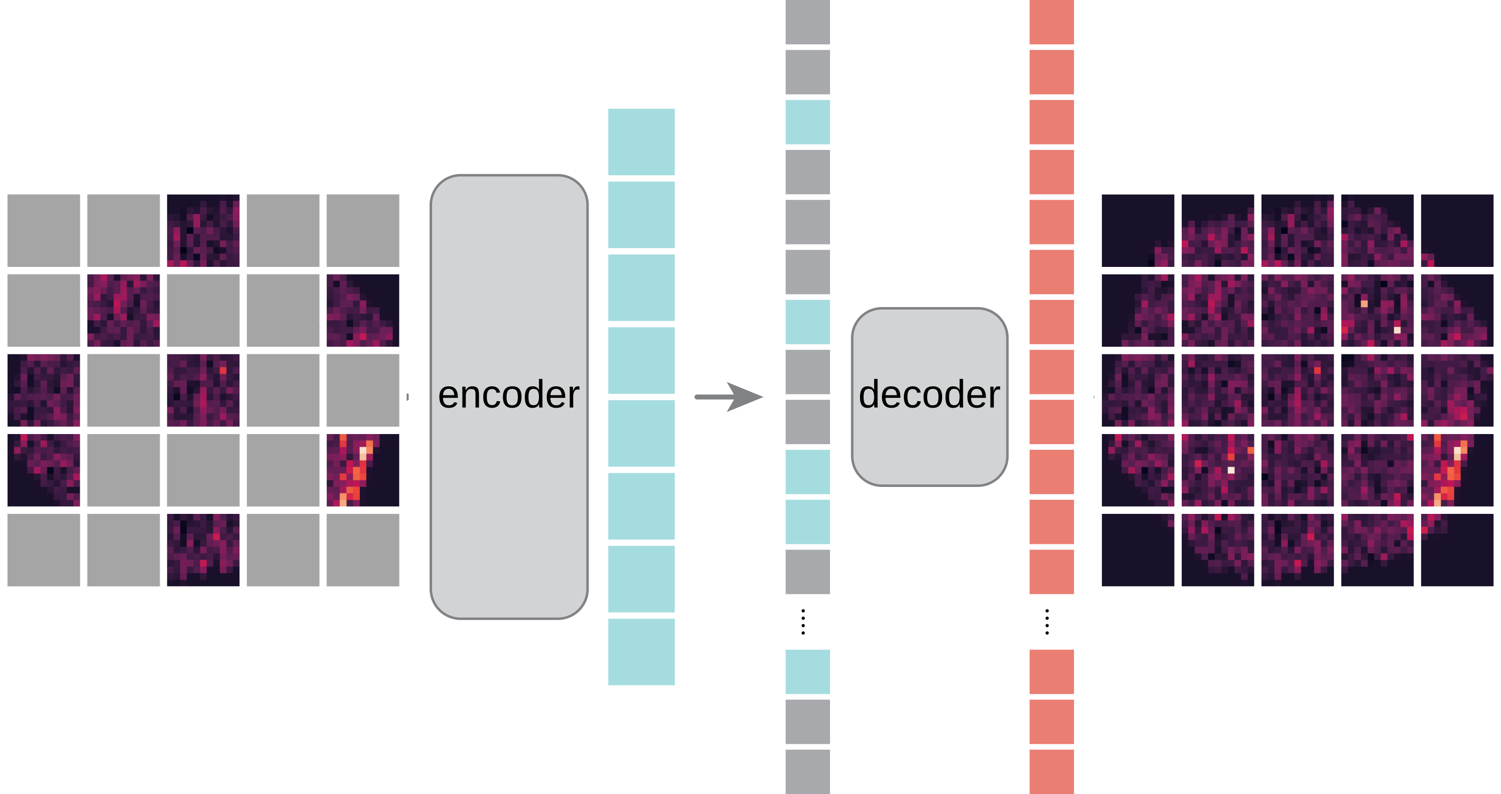
Kaiming He et al. [Masked Autoencoders Are Scalable Vision Learners.](https://arxiv.org/abs/2111.06377) 2021.
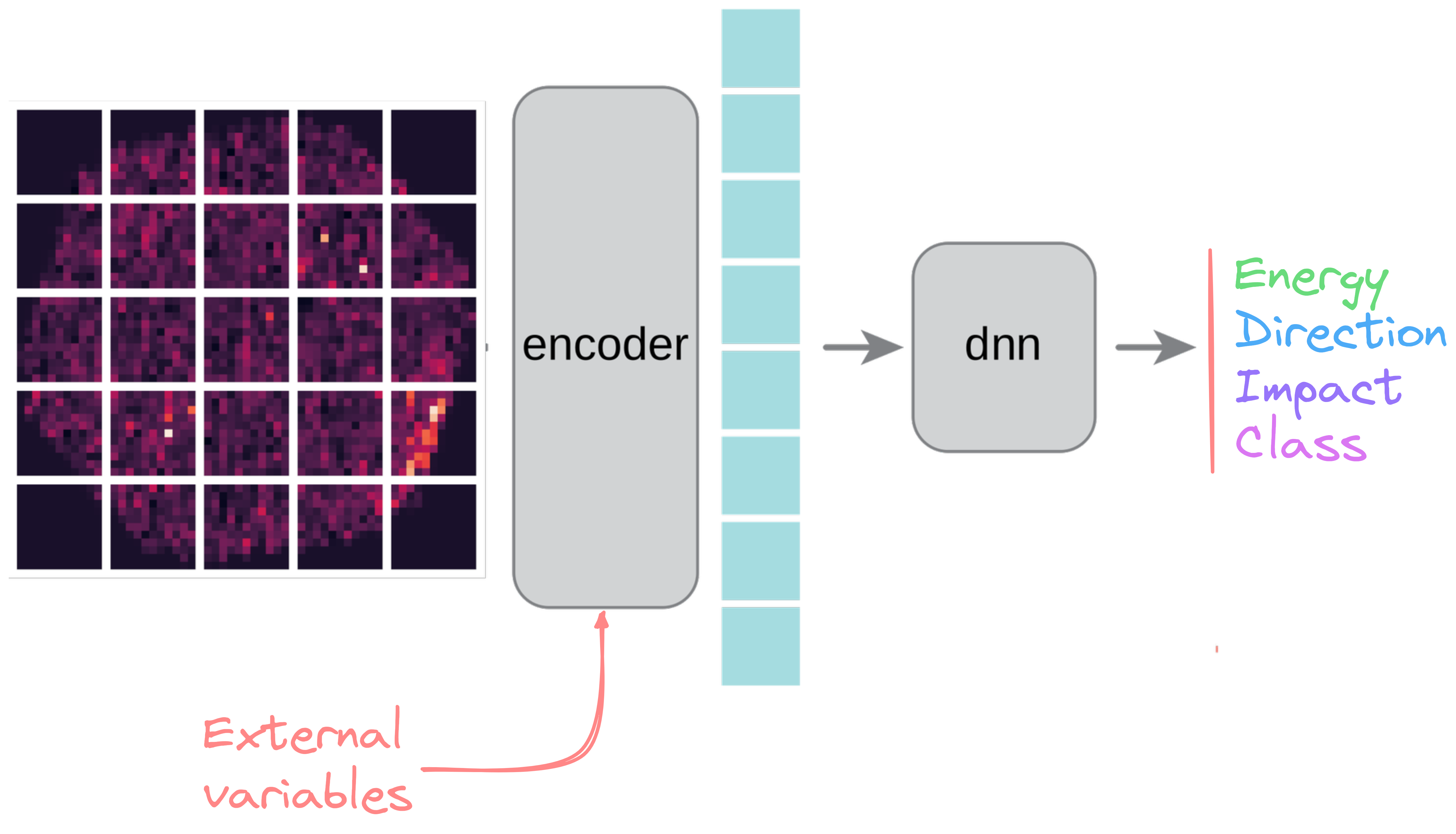
Event reconstruction example 1

Event reconstruction example 2

Event reconstruction example 3

The $\gamma$-PhysNet-Prime
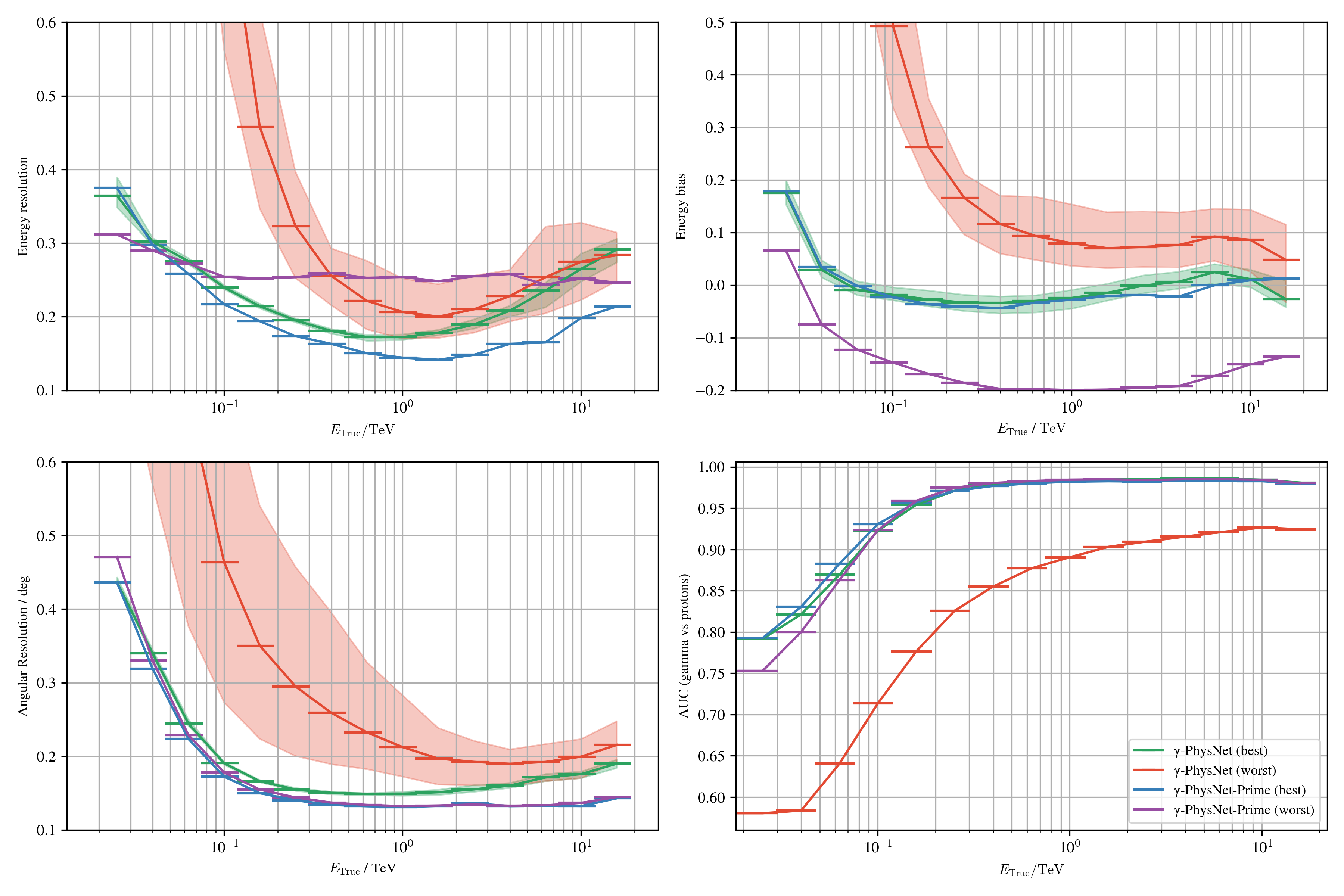
Results on Crab - $\gamma$-PhysNet-Prime


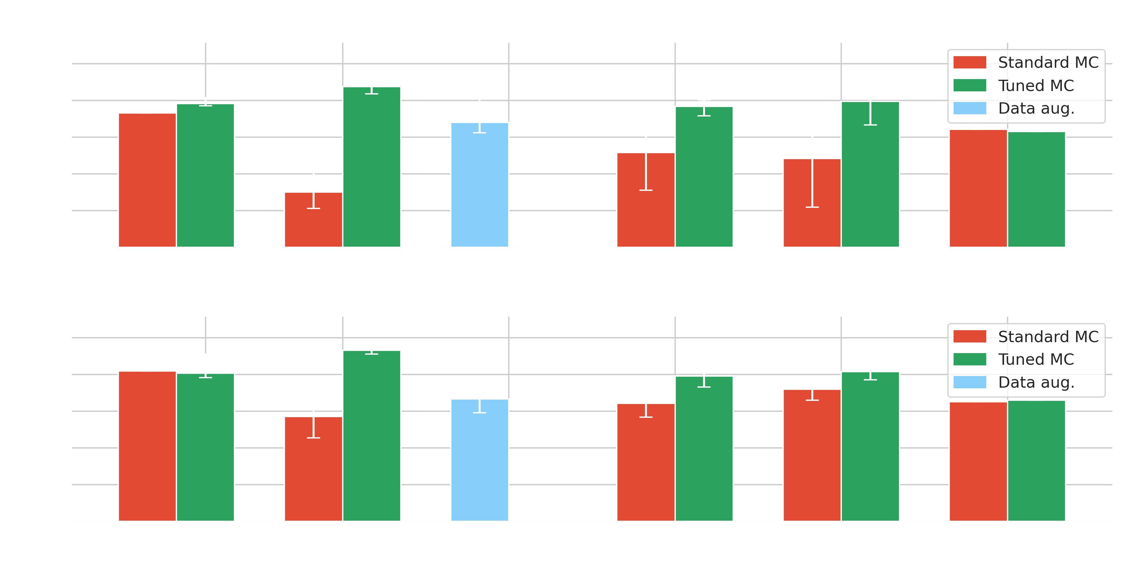


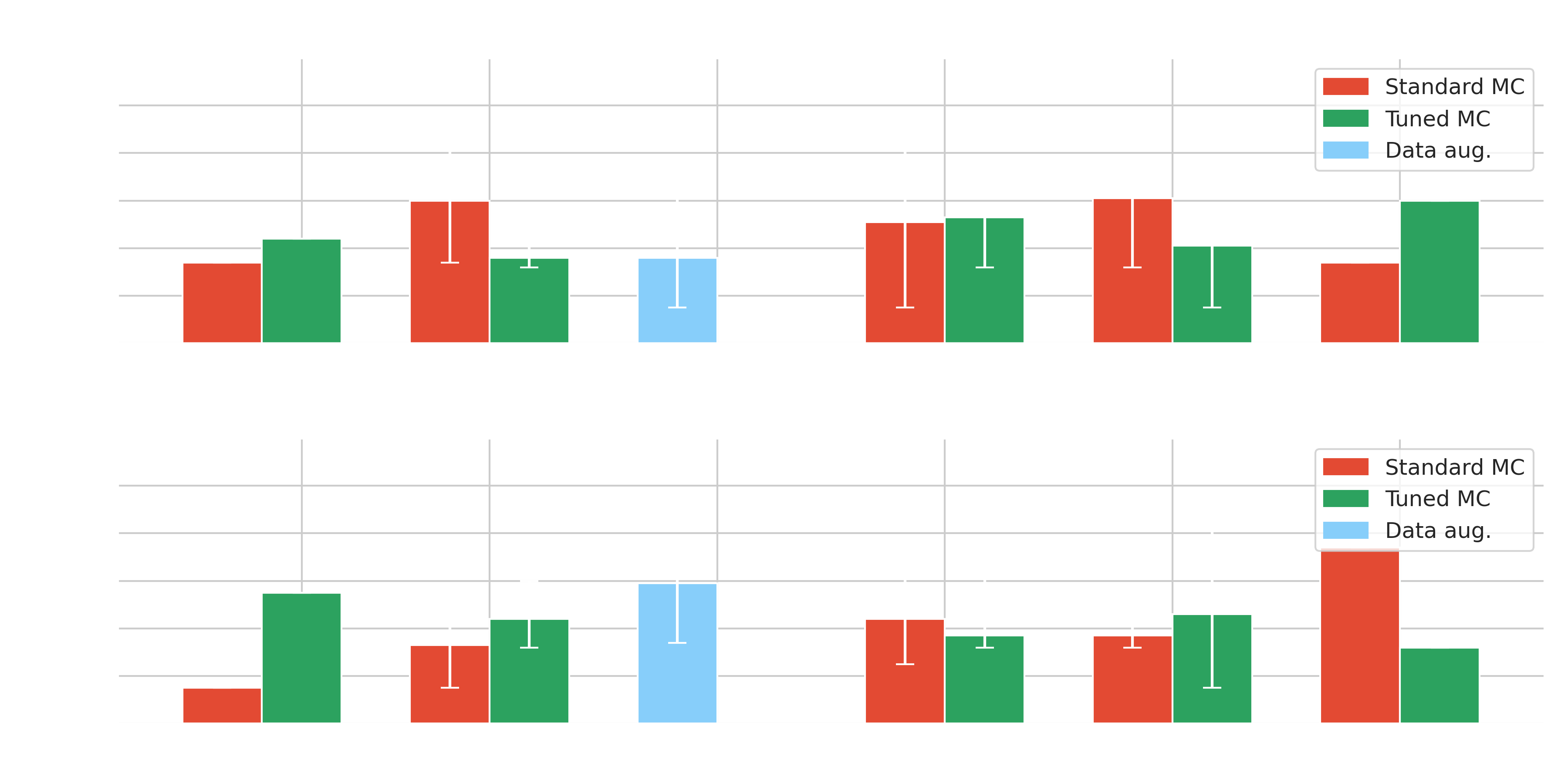


Conclusion and perspectives
Thesis contributions
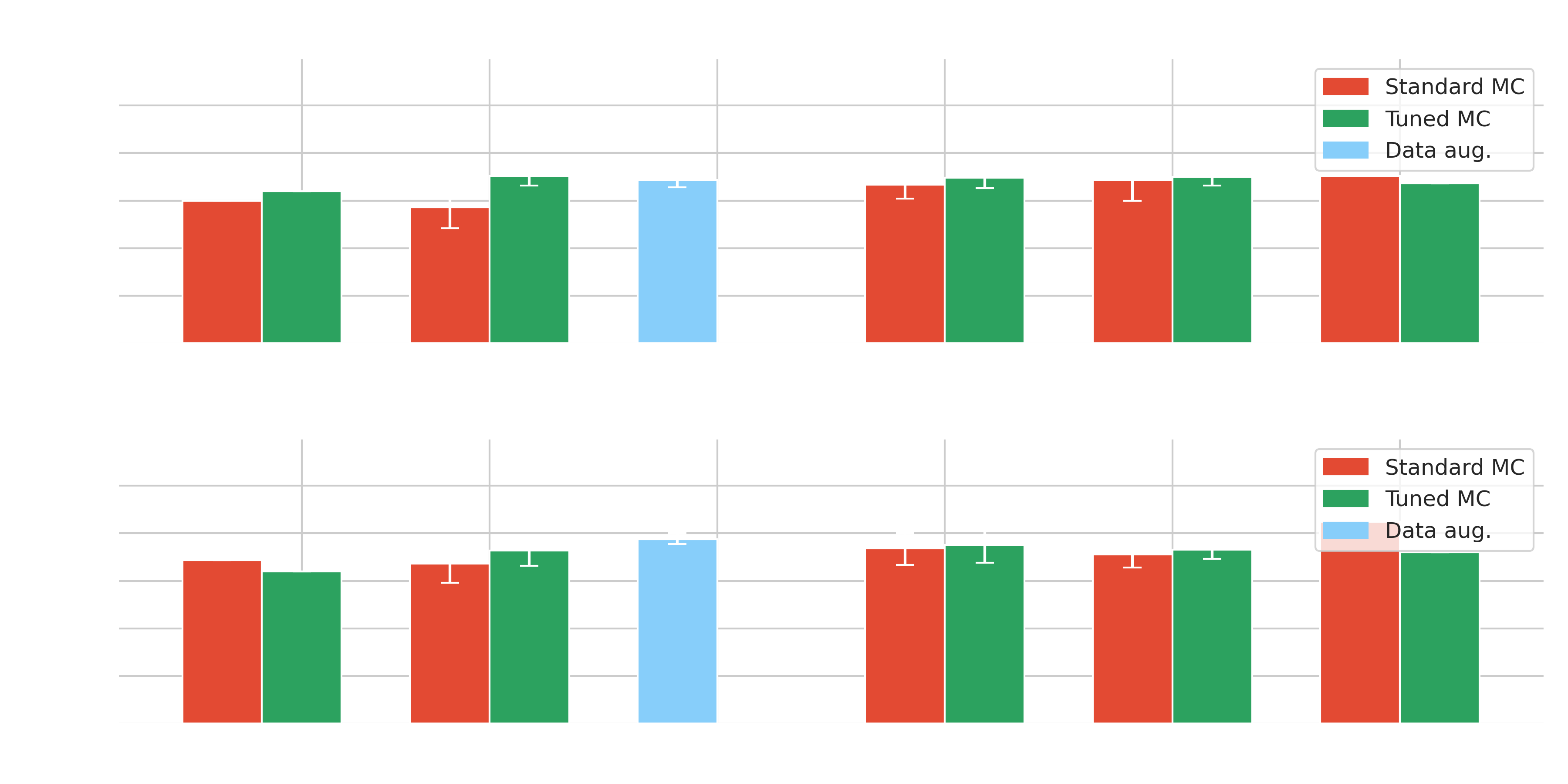
- Novel techniques (Information fusion, Unsupervised domain adaptation, Transformers) to solve simulations vs real data discreprency
- Tested on simulations, in different settings (Light pollution and label shift)
- Tested on real data (Crab), both moonlight and no moonlight conditions
- $\gamma$-PhysNet strongly affected by moonlight but not Hillas+RF
- Data adaptation, information fusion and Transformers increase the performance in degraded conditions without data adaptation
- Best results obtained on tuned data and on par with $\gamma$-PhysNet
- $\gamma$-PhysNet-CDANN allows to recover from label shift in simulations
- In our case, NSB is dominant compared to unkown differences
- Transformers are still under exploration and yield the best results on simulations
- A future comparison with ImPACT and FreePACT will be needed to fully evaluate our approaches
Perspectives
* Short term perspectives * Enhancement of the proposed methods * $\gamma$-PhysNet-CDANN with improved MTL * $\gamma$-PhysNet-CBN with pedestal image conditioning * $\gamma$-PhysNet-CBN with pointing direction conditioning * $\gamma$-PhysNet-Transformers combined with UDA * Improvement of the high-level analysis (e.g. compute FOM at different intensity bins) * Long term perspectives * Stereoscopic reconstruction and analysis (GNN, Transformers) * Explicability (Bayesian, GradCAM) * Real-time analysis
Publications
* A first proof-of-concept paper has been published at the CBMI 2023 international conference (Peer Reviewed) * A second proceeding has been accepted at the ADASS 2023 international (Proceeding) * A third paper submitted to the IEEE Transactions on Image Processing journal (Peer Reviewed) * A fourth paper, in preparation, to be submitted in the Astronomical Journal (Peer Reviewed)
Michaël Dell’aiera et al. [Deep unsupervised domain adaptation applied to the Cherenkov Telescope Array Large-Sized Telescope](https://dl.acm.org/doi/10.1145/3617233.3617279) in 20th International Conference on Content-based Multimedia Indexing 2023 Michaël Dell’aiera et al. [Deep Learning and IACT: Bridging the gap between Monte-Carlo simulations and LST-1 data using domain adaptation](https://arxiv.org/abs/2403.13633) in Astronomical Data Analysis Software & Systems 2023
Acknowledgments
![]()
![]()
![]()
![]()
![]()
![]()
![]()
![]()
![]()
![]()
![]()
![]()
Back-up
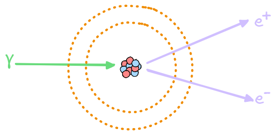
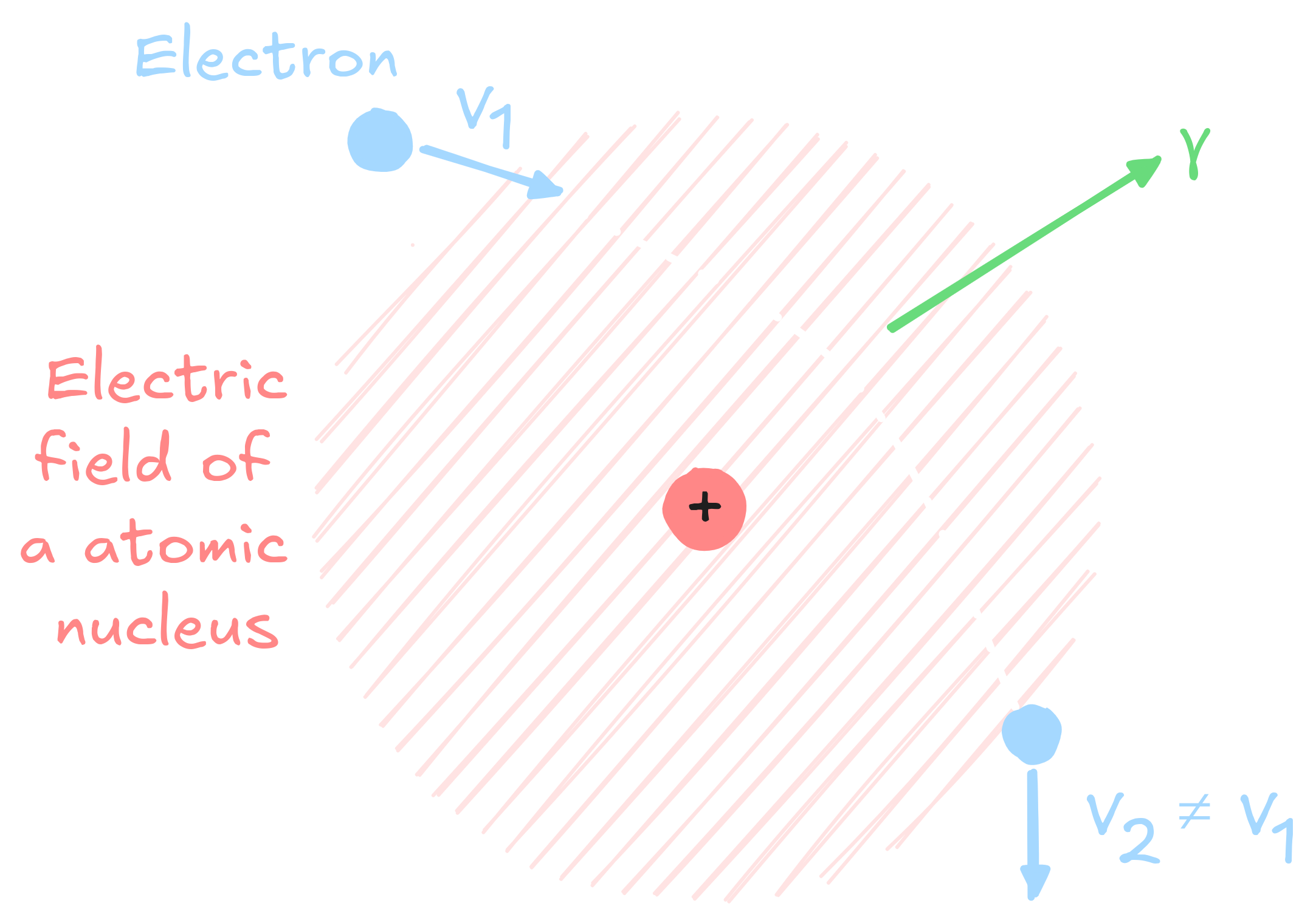
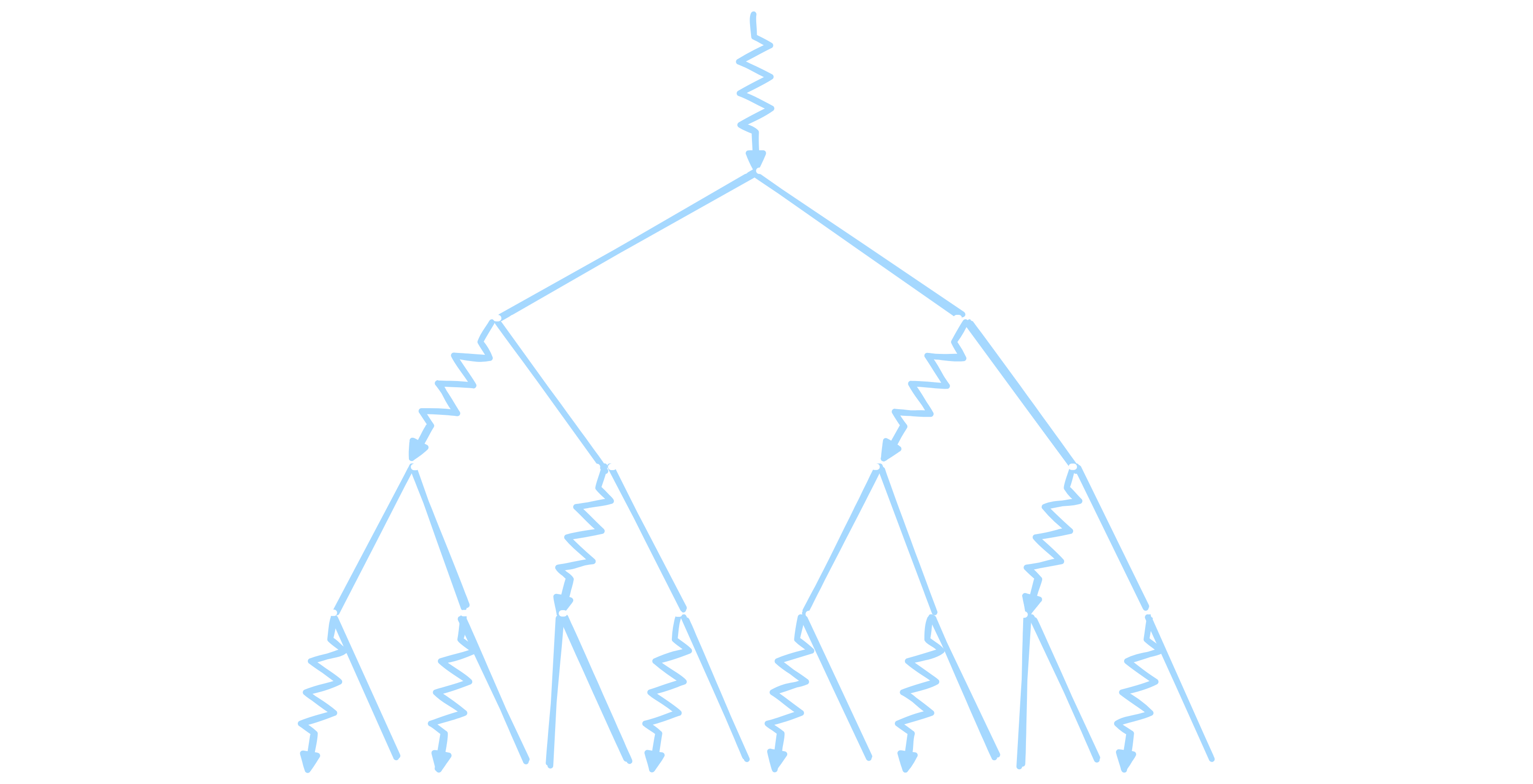
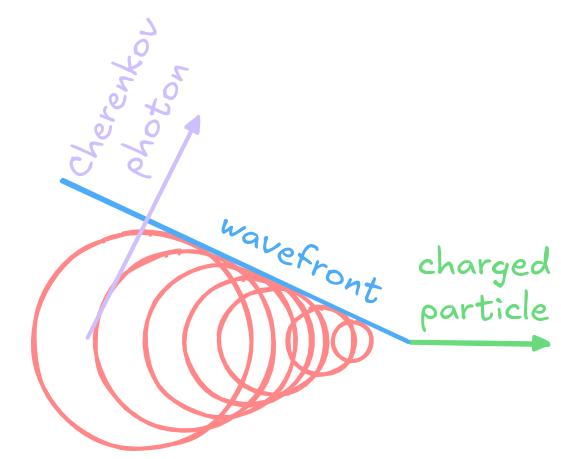
Physics processes
Significance
* Used to determine whether a signal is statistically significant above the background noise. * Significance of $5 \sigma$ or higher required to claim a valid detection of a signal.
\[ S = \sqrt{2} \left\{ N_{\text{on}} \ln \left[ \frac{1 + \alpha}{\alpha} \frac{N_{\text{on}}}{N_{\text{on}} + N_{\text{off}}} \right] + N_{\text{off}} \ln \left[ (1 + \alpha) \frac{N_{\text{off}}}{N_{\text{on}} + N_{\text{off}}} \right] \right\}^{1/2} \]* $N_{on}$ is the number of events in the signal region. * $N_{off}$ is the number of events in the background region. * $\alpha = \frac{T_{\text{on}}}{T_{\text{off}}}$ is the ratio of the exposure times or areas between the signal and background regions
T. -P. Li and Y. -Q. Ma. [Analysis methods for results in gamma-ray astronomy.](https://adsabs.harvard.edu/full/1983ApJ...272..317L) In: 272 (Sept. 1983), pp. 317–324
Reconstruction bias
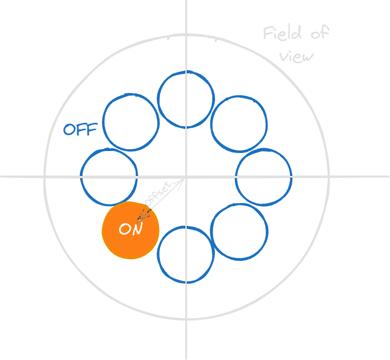
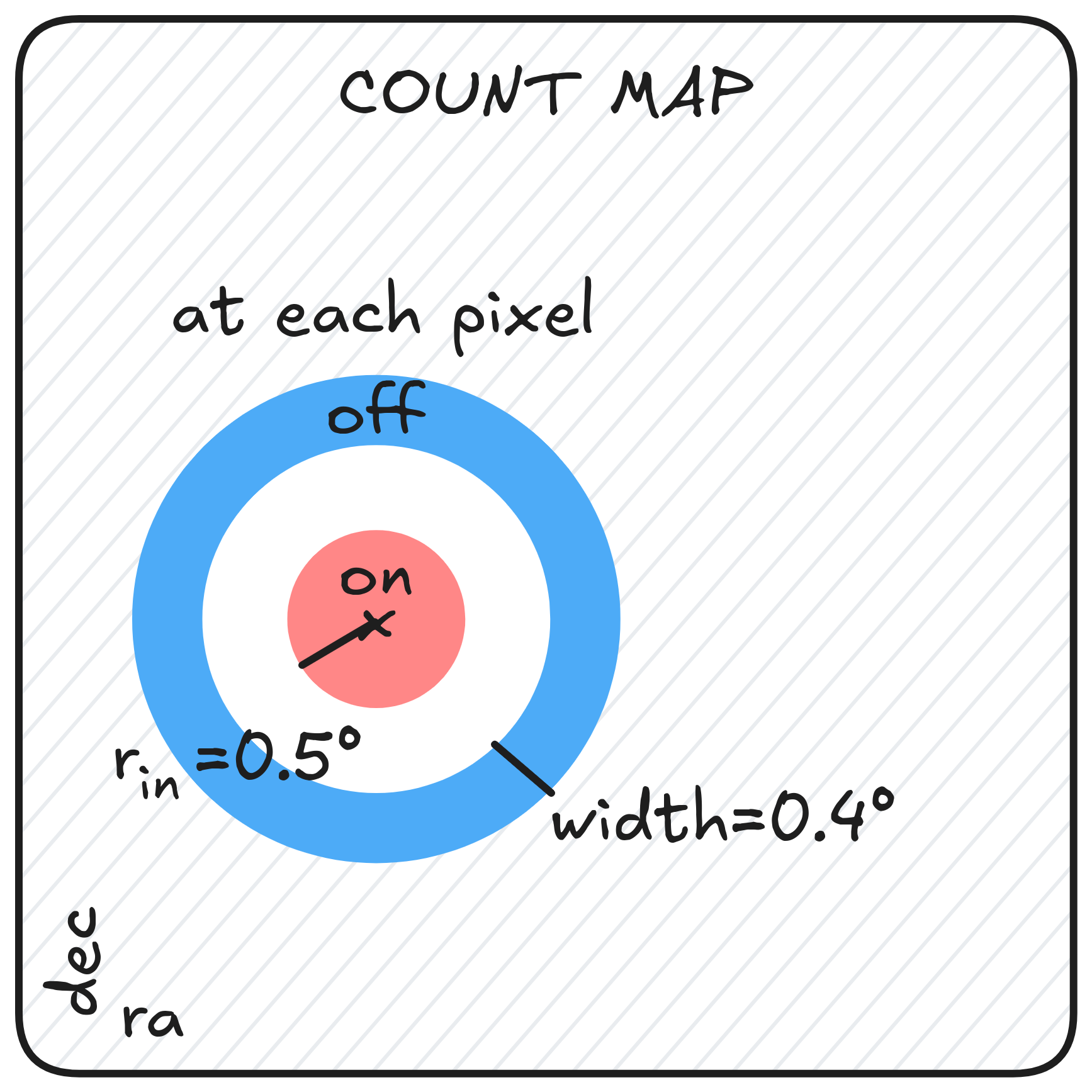
* For each pixel * a ON region of $r_{in}=0.2^\circ$ is created * a donut-like OFF region of $w=0.4^\circ$ is created * we count the number of events $N_{on}$ and $N_{off}$ * we calculate the significance $\sigma=\frac{N_{on}-\alpha N_{off}}{\sqrt{\alpha (N_{on} + N_{off})}}$ * $\alpha=\dfrac{\int_{ON} EffA(x,y,E,t)dxdydEdt}{\int_{OFF} EffA(x,y,E,t)dxdydEdt}$ * EffA obtained using Mathieu de Bony's background model * On the significance map * Combined significance in regions * Take the highest significance as the reconstructed position
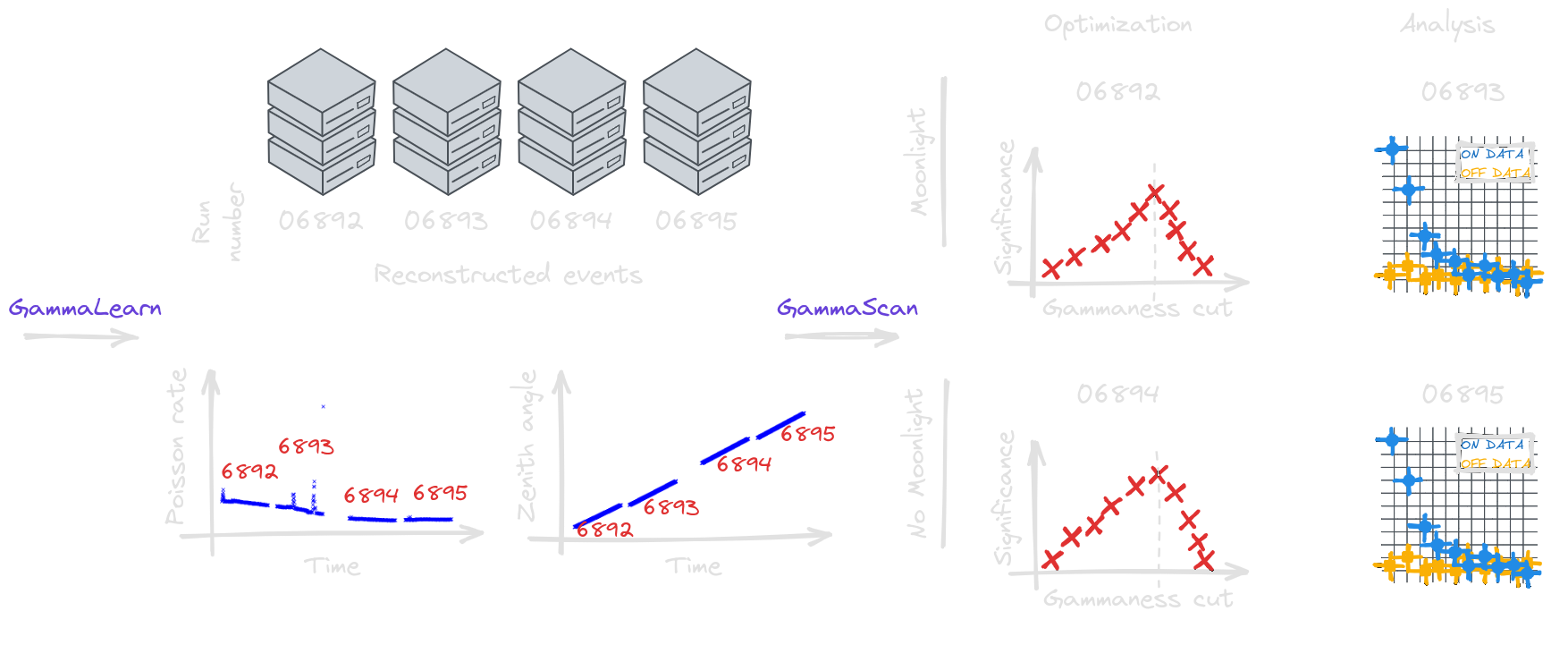
Optimal cuts
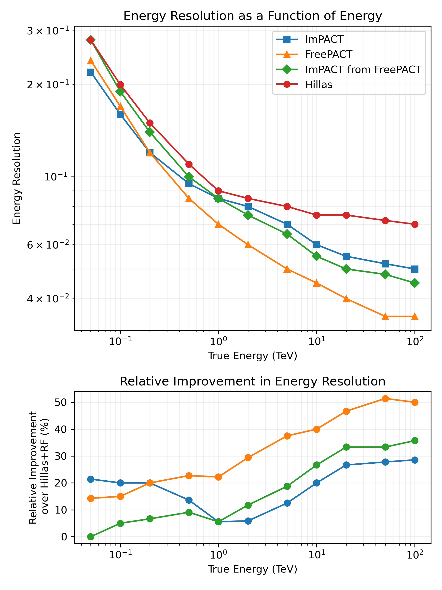
Method comparison
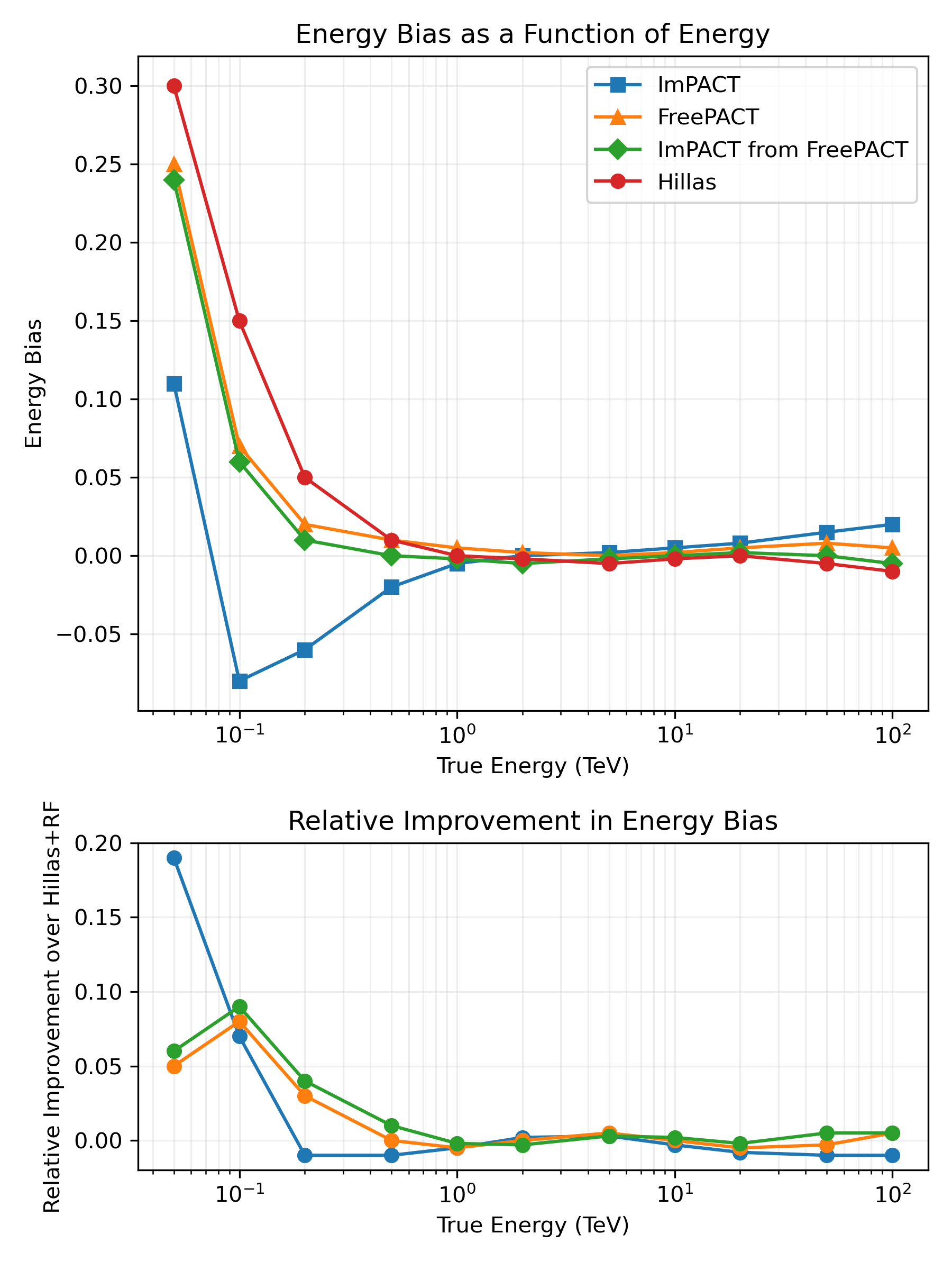
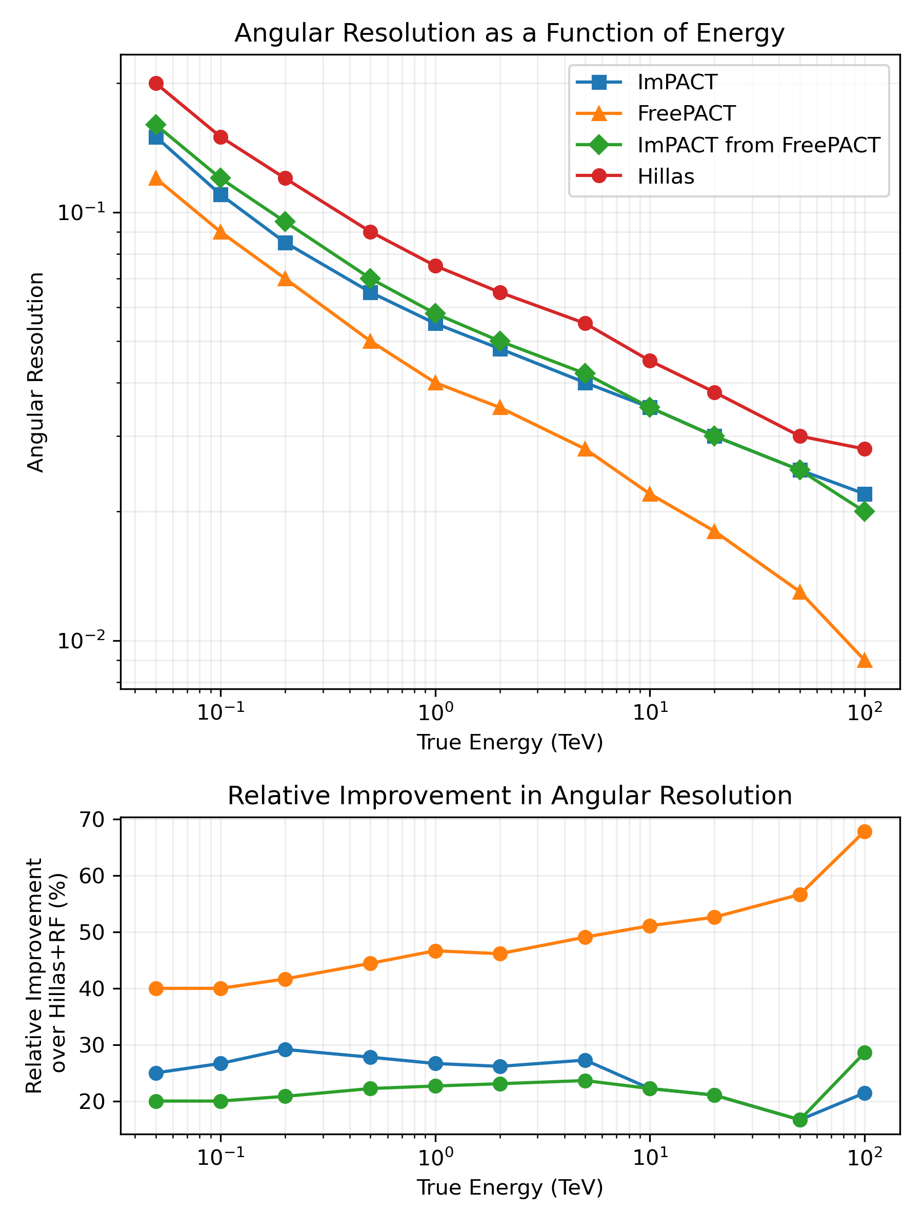
Method comparison
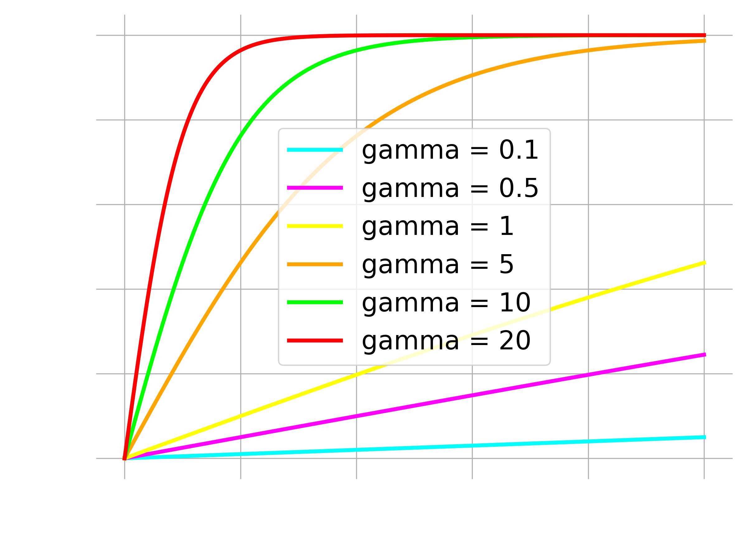
Gradient Layer
Domain conditioning

Xiaofeng Liu et al. [Adversarial Unsupervised Domain Adaptation with Conditional and Label Shift: Infer, Align and Iterate.](https://arxiv.org/abs/2107.13469) 2021.
Litterature exploration
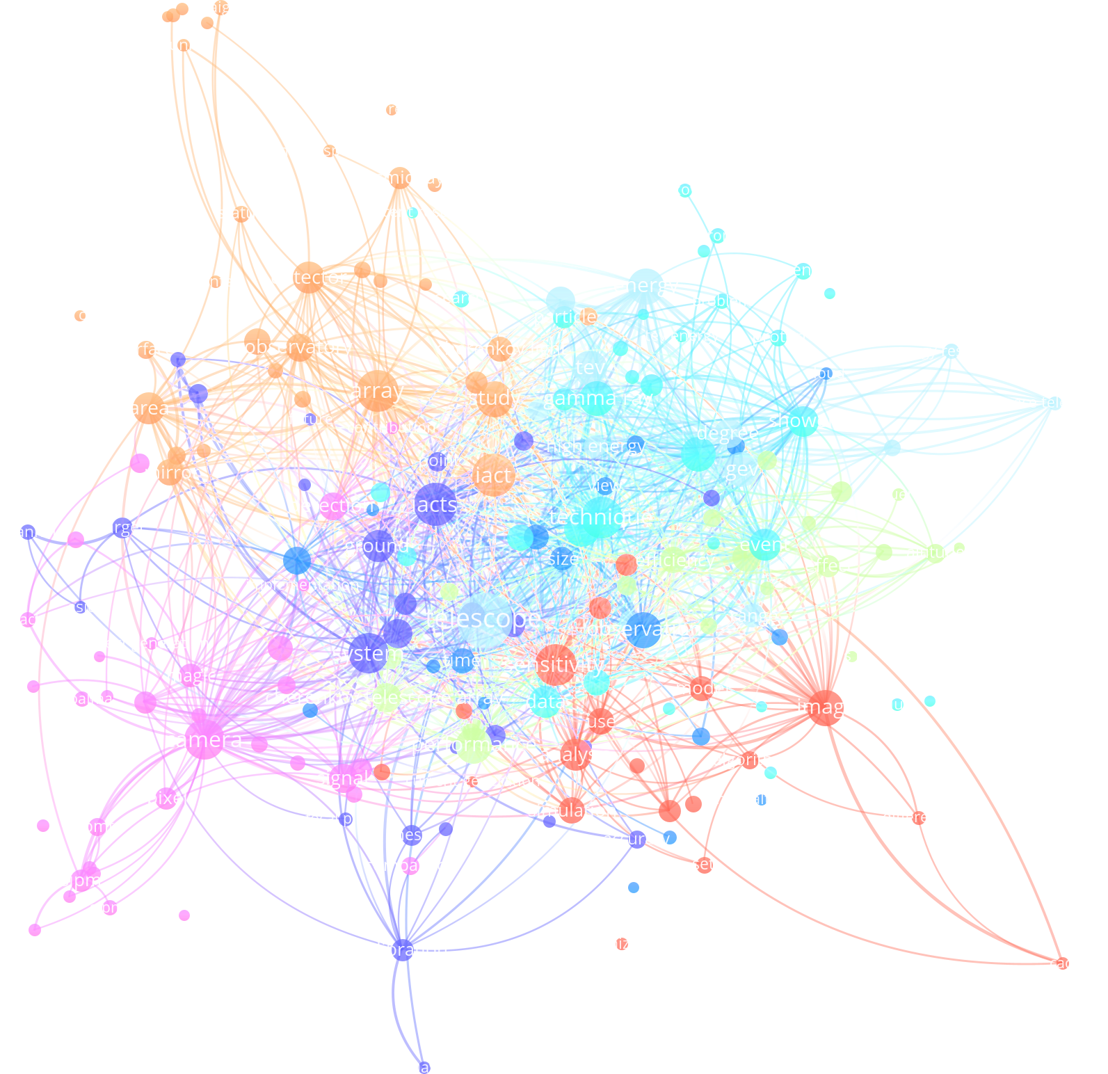
Results on Crab - $\gamma$-PhysNet-Prime
| Methods | Significance | Position bias | # Seeds | |
|---|---|---|---|---|
| Standard | Hillas+RF | 18.3 (18.3) |
0.034 (0.034) |
1 |
| γ-PhysNet | 7.54 (10.7) | 0.060 (0.034) | 5 | |
| γ-PhysNet-DANN | 12.9 (17.0) | 0.051 (0.015) | 5 | |
| γ-PhysNet-CDANN | 12.1 (16.1) | 0.061 (0.032) | 5 | |
| γ-PhysNet-Prime | 16.1 (16.1) | 0.034 (0.034) |
1 | |
| Tuned | Hillas+RF | 19.5 (19.5) | 0.044 (0.044) | 1 |
| γ-PhysNet | 21.9 (22.9) |
0.036 (0.032) |
5 | |
| γ-PhysNet-DANN | 19.2 (20.1) | 0.053 (0.032) | 5 | |
| γ-PhysNet-CDANN | 19.9 (22.4) |
0.041 (0.015) | 5 | |
| γ-PhysNet-Prime | 15.8 (15.8) | 0.060 (0.060) | 1 | |
| γ-PhysNet-CBN | 17.0 (20.3) | 0.036 (0.015) | 4 |
| Methods | Significance | Position bias | # Seeds | |
|---|---|---|---|---|
| Standard | Hillas+RF | 20.5 (20.5) |
0.015 (0.015) |
1 |
| γ-PhysNet | 14.3 (16.1) | 0.033 (0.015) | 5 | |
| γ-PhysNet-DANN | 16.1 (16.8) | 0.044 (0.025) | 5 | |
| γ-PhysNet-CDANN | 18.0 (19.3) | 0.037 (0.032) | 5 | |
| γ-PhysNet-Prime | 16.3 (16.3) | 0.074 (0.074) | 1 | |
| Tuned | Hillas+RF | 20.5 (20.5) | 0.055 (0.055) | 1 |
| γ-PhysNet | 23.1 (23.8) |
0.044 (0.032) | 5 | |
| γ-PhysNet-DANN | 19.8 (22.3) | 0.037 (0.032) | 5 | |
| γ-PhysNet-CDANN | 20.4 (22.5) | 0.046 (0.015) | 5 | |
| γ-PhysNet-Prime | 16.5 (16.5) | 0.032 (0.032) |
1 | |
| γ-PhysNet-CBN | 16.7 (18.7) | 0.059 (0.034) | 4 |